Preprocessing before a PTA-$k$modes

Preprocessing such as centring and/or scaling enables the analysis to focused on a chosen variation of interest. It can sometimes be a solution to the problem of subject effect and outlier effects (effects occurring in the pharmaco-EEG data, see [11]). Centring and/or reducing variables before analysis is common in multivariate analysis such as PCA. Usually centring is seen as a simple statistical model focussing on residuals from a regression model and has connections with algebraic and geometrical properties, such as being the projection onto the orthogonal of the subspace generated by the regressors. With this interpretation and leaving, aside the statistical sampling who generated the data, it is possible in fact to centre and/or reduce on any mode or combined mode of our multi-entries data. Remembering the structure of our data described at the beginning of section 4, the question is now ``what are we looking for?" which should guide our decisions with respect to centring/reducing. The question could be formulated as ``what are we not interested in?". At first sight the answer to this one is subject differences, but also the interactions of subject and the other ``dimensions". If the data is firstly whole centred, centring and removing effects (as in ANOVA) are linked. To understand this point consider the problem in two modes with $x$ whole centred, i.e. $\bar{x}=x_{..}=\sum_{ij} x_{ij}=0$ :

$$x^{c}_{ij} = x_{ij} -x_{.j}$$

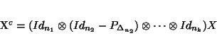
is called in [20] centring across the first mode, and is equivalent in ANOVA language to remove the effect of the second mode. This is the reason why one usually centres across the mode of interest. It is possible to give an algebraic expression to this transformation : with $X$ a tensor of order k when centring across say the second mode, $X$ is transformed to :

$$X^{c}=(Id_{n_1}\otimes(Id_{n_2}-P_{\Delta_{n_2}})\otimes \cdots \otimes Id_{n_k})X$$ (13)

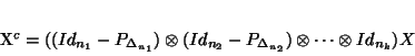
where $P_{\Delta_{n_2}}$ is the orthogonal projector onto the vector $\Delta_{n_2}= ^t(1,1, \ldots,1)$ of length $n_2$, and $Id_{n_u}$ is the identity operator onto $\mathbb{R}^{n_u}$ . The expression (13) is using the tensor product of linear operators (see also next section) which is isomorphic to the Kronecker product of their matrices (for any given basis choices). Performing a double centring say across the first mode and across the second mode can be written :

$$X^{c}=((Id_{n_1}-P_{\Delta_{n_1}})\otimes(Id_{n_2}-P_{\Delta_{n_2}})\otimes \cdots \otimes Id_{n_k})X$$ (14)

It easy to show that it is equivalent to perform the two single centring one after the other. Care is needed in multiple centring and /or reducing involving centring across slices (2 modes varying) as well, as one can cancel or slightly modify the other centring. This is because doing successively mode centring and slice centring may break the tensorial structure. A simple example involving only slice centring and showing a broken tensorial structure would be to centre across slice [mode 1 and mode 2] and then across slice [mode 2 and mode 3]! For such situations, iterative centring and scaling can be also be thought as for the PARAFAC method in [20] but this preprocessing algorithm may then become a true modelling part of the analysis for which interpretation and analysis of the explained part ($X-X^c$) may be needed. For EEG data it is possible to have this ANOVA like approach for all the entries (at least when looking at absolute energies) as one can consider the data as a measure of the EEG amplitude on the subjects at the repeated conditions : electrodes, frequency bands, time, and doses. Note the structure of the data ensures a balanced design and so orthogonality of factors for the ANOVA. The problem in using this ANOVA approach is that if distributions are not normal with small variances, a factor effect measured with means will not be completely removed, i.e. the variation left may be still important. Others structures than the one giving the mean model can be considered for an entry $h$, the formula (14) can be reformulated replacing the model $\Delta_{n_h}$ by the appropriate $G_{n_h}$ (a ``design" describing the structure usually including $\Delta_{n_h}$) .

Figure 4: PTA-$4$modes of all bands (absolute energies) for verum versus placebo versus first baseline: $1^{st}$ Principal tensor (a) original data, (b) subjects scaled to unit, (c) globally-modified data (d) levels-modified data; (preprocessing b, c, and d explained in the text).

[Original data]

[Subject scaled data]

[globally-modified data]

[levels-modified data]

Scaling (or reducing) variables is commonly used when the variable units are not the same. For EEG measurements subjects can be thought to have their own units. Global subject differences in location and in variability are not of interest for our purpose, so reducing their variability to the same unit would also improve the analysis. Unfortunately centring or removing effects does not insure vanishing outliers, but sometimes successfully diminishes the variability induced by their presence so that it appears in a less important (lower singular value) Principal Tensor. A complete illustration of this fact is shown in [12]. On fig.4 a comparison of the first principal tensor obtained from the data [dose*subject $\times$lead $\times$ time $\times$band] with different preprocessing is shown . To modify the data using the ANOVA approach it is possible to remove interactions of each factor (mode) with subjects globally or by levels of other factors. For example on the subject scaled data was removed : subject.dose by time and band, subject.band by time and dose, subject.time by band dose, and, subject.electrode by band dose. Notice the first interactions are then computed on the electrode units, and the last one is computed on time units. This way of proceeding can make more sense than computing these interactions globally on the rest of the units, and actually provided better results. A verification was done in comparing full ANOVA models (the subject factor being the experimental units) respectively on the subject scaled data, the globally-modified data (interactions and main subject effect removed), the levels-modified data (as before but by levels). We obtained as explained respectively : $5\%$, $13\%$, and $35\%$, which means some unwanted variation in the data were successfully removed.