Non-Identity metrics in PTA-$k$modes

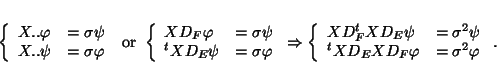
The general method of SVD-kmodes can be performed with non-identity metrics. This means that inner products can be considered weighted (diagonal metrics) or cross-weighted (non-diagonal metrics). The whole algebraic setup used at the beginning of the paper is the same if one understands the contracted product (operation ..) as containing the metrics. For example, equations (5) expressing the classic SVD become :

$$\sigma_1 = \max_{{\scriptstyle \begin{array}{l } \scriptstyle \left\Vert \ps... ...yle \left\Vert \varphi \right\Vert _F =1 \end{array}}}A..(\psi \otimes \varphi)$$

$$= A..(\psi_1 \otimes \varphi_1) \quad (\mbox{ in tensor form})$$

$$= ^t\psi_1 D_E A D_F \varphi_1 \quad (\mbox{ in matrix form});$$ (16)

where spaces $E$ and $F$ have now respectively the metrics $D_E$ and $D_F$ (instead of the identity metrics). The only change is in the last expression (matrix form) because the metrics are ``included" in the contracted product operation as well as in the norms (as defined from the inner product) ; equation (6) is as well :

$$\left\{ \begin{array}{ll} X..\varphi & =\sigma \psi ... ... ^tXD_EXD_F\varphi & =\sigma^2 \varphi \end{array} \right. .$$ (17)

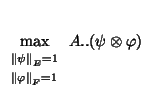
Consideration of metrics offers flexibility to the analysis. For example with two modes it is classical to recognise a discriminant analysis as a SVD on the projected data with $\Sigma^{-1}$ (the inverse of the covariance matrix) as metric on the space defined by the variables or as a SVD of the original data with $W^{-1}$, the inverse of the within covariance matrix. Roughly speaking, when looking for ``best directions", directions of high within variation have a lower weight than the other directions (see also [2] when the group structure is not known). Another good example of non-identity metrics is also in the next section, correspondence analysis. Nonetheless the method offers the possibility only of decomposed whole space metrics, i.e. of the form:

$$M_{E_1} \otimes M_{E_2} \otimes M_{E_3} \ldots \otimes M_{E_k}$$ (18)

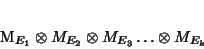
where every metrics as algebraic object (self-adjoint linear operator) is confounded with its definite or semi-definite positive matrix representation (like $X$ as tensor and array or vector). The tensor product operation is the one for linear operators (see also [4]). It is left with the same notation (as for vectors) because it is possible to confound the algebraic notation and arithmetic, as well . This is because it becomes the Kronecker tensor product sometimes called the outer product which operates either on vectors or matrices. One must note that (18) is a linear operator onto the whole space,which operates separately onto every space defining the tensor space (this is in fact the definition of the tensor product of linear operators). Arithmetically and computationally this can be written:

$$(M_E \otimes M_F \otimes M_G)(Y) = (M_E \otimes M_F \otimes M_G)(Y)$$ (19)

$$= (M_E \otimes M_F \otimes M_G)(\sum_u e_u \otimes f_u \otimes g_u)$$

$$= \sum_u (M_E e_u) \otimes (M_F f_u) \otimes (M_G g_u)$$

Without knowing the decomposition of $Y$, this last expression cannot be used, nonetheless isomorphism properties within multilinear maps (tensor) can be used to perform successively the different operators (e.g. $Y\in E\otimes F \otimes G \sim \mathcal{L}(E^*; F \otimes G)$ then 19 is equivalent to $( M_F \otimes M_G)(Y \circ M_E )$ where $\circ$ stands for composition of applications or matrix multiplication). The contraction product includes the metrics using this property and could also have been understood as a canonical contraction product (without metrics) of the transformed tensor (the contracting one) by the metric operators, i.e. the canonical contraction would be using only the dual product instead of the inner product:

$$Y..z=Y.._c (M_E z)=[Y \circ M_E ] .._c z$$ (20)

What is a good choice of metrics for pharmaco-EEG studies ? Generally Choices are geared towards ``elimination" of unwanted variation, such as in discriminant analysis one do not want to relate the within group variation. For pharmaco-EEG data it would be interesting to eliminate natural variation of bands and electrodes as well as within dose variation. To achieve estimation of natural variation, enough placebo observations or better some ``null" data on the subjects studied are needed. Metric choice and their estimation is a key issue in multidimensional and/or multiway analysis particularly for this kind of data and deserves more attention (see [15]).