Next: SVD-kmodes for and
Up: Multiway multidimensional data reduction
Previous: Multiway multidimensional data reduction
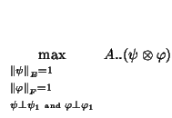
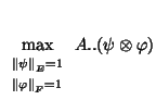
The first singular value of a data matrix  is :
is :
 is termed first principal component,
  first principal axis,
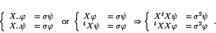
 will be called first principal tensor. Solving the problem associated
with this maximisation leads to transition formulae and then to the classical eigenequations where
, and
will be called first principal tensor. Solving the problem associated
with this maximisation leads to transition formulae and then to the classical eigenequations where
, and  are the first eigenvectors and eigenvalue of the respective
symmetric operators:
are the first eigenvectors and eigenvalue of the respective
symmetric operators:
 |
(6) |
To compute the solutions one can either use the eigenequations or execute an iterative algorithm using
the transition formulae. To find the second and further solutions it is added an orthogonal
constraints (uncorrelated vectors) onto the  and
and  :
:
Here with  , the orthogonality constraint can be written either
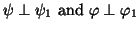 , or
, or
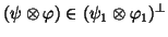 , or
with the subspace termed orthogonal-tensorial of the first principal tensor
, or
with the subspace termed orthogonal-tensorial of the first principal tensor
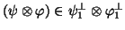 .
.
The SVD is then written as an orthogonal decomposition of ,
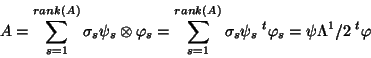 |
(8) |
in tensor form, or in vector form, or in matrix form. Note that here (for 2 modes) the collection of
 and the collection of
  give also orthogonal systems within the respective spaces ;
that will not be generally the case for
give also orthogonal systems within the respective spaces ;
that will not be generally the case for  modes.
Next: SVD-kmodes for and
Up: Multiway multidimensional data reduction
Previous: Multiway multidimensional data reduction
Didier Leibovici
2001-09-04