Next: SVD within tensor algebra
Up: tr00dl2
Previous: Shortcomings of current statistical
The aim of this section is to explain the basics of the SVD-kmodes method as an extension of
SVD. The presentation can be limited to  and
and  as the case
  is then a
straightforward extension. Further details are in [16]. First of all the development
of this generalisation of the SVD (Singular Value Decomposition) is described within tensor
algebra framework in finite dimension. It enables us to extend matrix algebra calculus in an easy
way. A tensor of order one is a vector, a tensor of order two is a matrix, a tensor of order three
is three-way array etc...
is then a
straightforward extension. Further details are in [16]. First of all the development
of this generalisation of the SVD (Singular Value Decomposition) is described within tensor
algebra framework in finite dimension. It enables us to extend matrix algebra calculus in an easy
way. A tensor of order one is a vector, a tensor of order two is a matrix, a tensor of order three
is three-way array etc...
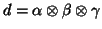
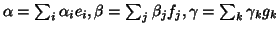
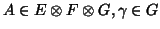
Let
 ,
,
 , and
, and
 be the canonical bases respectively
of
be the canonical bases respectively
of  ,
,  and
and  ; with
  and
and  let us define the
bilinear map
let us define the
bilinear map  by:
by:
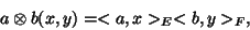 |
(1) |
(where  is the inner product in
  ) ; consider now the canonical bilinear maps built
with the
) ; consider now the canonical bilinear maps built
with the  and
and  , they constitute a base of a space noted
  the tensor product
of the spaces and
the tensor product
of the spaces and  . Without going further into algebraic concepts, notice that because of
symmetry in equation (1)
. Without going further into algebraic concepts, notice that because of
symmetry in equation (1)  can be considered as a linear map onto , so
that one has the universal property of the tensor product: transforming a bilinear map
(multilinear in general) into a linear map.
An
can be considered as a linear map onto , so
that one has the universal property of the tensor product: transforming a bilinear map
(multilinear in general) into a linear map.
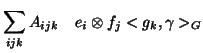
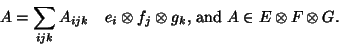
An  matrix
  of elements
 , can be written algebraically,
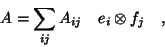 |
(2) |
and is
said to belong to the space , tensorial product of the spaces and
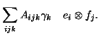
1. Notice that the array, the linear map
associated, the tensor are noted because of isomorphisms. In the same manner a three-way array
 of elements
 , can be written algebraically,
 |
(3) |
The vectors of the space
 with the form
 (where
 ) are called decomposed tensors, and are said to be of rank one - a sum of
  linearly
independent decomposed tensors would give a rank tensor-2. To finish
with basic tools of tensor algebra, let us also introduce the generalisation of a product of
a vector by a matrix: the product of vector (or a tensor) by a tensor, also called contraction
and noted ``..". For example let
linearly
independent decomposed tensors would give a rank tensor-2. To finish
with basic tools of tensor algebra, let us also introduce the generalisation of a product of
a vector by a matrix: the product of vector (or a tensor) by a tensor, also called contraction
and noted ``..". For example let
 , then
 with:
with:
Arithmetically this can be seen considering as a matrix with  rows and
  columns, then
calculating the image of
columns, then
calculating the image of  by this matrix gives a representation of
  . Note that
 is the inner product between the tensors
 .
.
Subsections
Next: SVD within tensor algebra
Up: tr00dl2
Previous: Shortcomings of current statistical
Didier Leibovici
2001-09-04