A first analysis

Before going further the investigation of interesting choices to perform the analysis, let us have a glimpse at the kind of results the PTA-$k$modes provides on our actual data.
Using the statistical method of [3], briefly described in section 2, results reported from an independent body were summarised as follow:

``The most consistent treatment effects observed are a dose dependent increase of the total energy with a peak measured around time 2.5-3h post-dosing, and a spectral redistribution of energy in favour of the $\delta$ frequency band. These effects are detected already after 0.5-2h and are maximal around 3h post-dosing, as all the other significant effects observed. In addition to the increase observed for the $\delta$ band, a selective increase of the $\beta_1$ band and a reduction of the $\alpha_1$ band is observed around 3h post-dosing."

In order to try to replicate these results, a first analysis has been made only on total band with a time dimension, an electrodes dimension, and a subject*dose dimension.

Table 1: PTA-$3$modes of total energy for verum versus placebo versus 1$^{st}$ baseline: listing of the decomposition up to the second $k$modes and associated solutions.

***********************************************
  PTA-3modes  dim x (36) dim y (28) dim z (9)
  data    dose*sujets    electrodes   time
  pdy2833
***********************************************
total band day 1 vs bl: verum vs plb
-----------------------------------
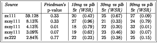
  Decomposition after Prin.tens 222
          explained 96.314621 %
-----------------------------------
Values                PCT      PCTloc
 vs111    10.264229   59.128 %   .     vs222    2.2504552   02.842     .
  Xvs11   10.264229     .      98.65    Xvs11   2.2504552     .      82.49
  Xvs11   1.0391565   00.606   01.01    Xvs11   0.8390228   00.395   11.47
  Xvs22   0.3847897   00.083   00.14    Xvs22   0.4463147   00.112   03.24
  Xvs33   0.2981522   00.050   00.08    Xvs33    0.319963   00.057   01.67
  Xvs44   0.2686759   00.041   00.07    Xvs44   0.1950296   00.021   00.62
  Xvs55   0.1569165   00.014   00.02    Xvs55   0.1361017   00.010   00.30
  Xvs66   0.1193496   00.008   00.01    Xvs66   0.1151387   00.007   00.22
  Xvs77   0.1046065   00.006   00.01    Xvs77   4.105E-17   00.000   00.00
  Yvs11   10.264229     .      74.28    Yvs11   2.2504552     .      59.11
  Yvs11   3.8071438   08.135   10.22    Yvs11   1.0813549   00.656   13.65
  Yvs22   2.7134542   04.132   05.19    Yvs22   0.9753945   00.534   11.10
  Yvs33   2.3470325   03.092   03.88    Yvs33   0.7212513   00.292   06.07
  Yvs44   2.2247245   02.778   03.49    Yvs44   0.6557279   00.241   05.02
  Yvs55   1.4559578   01.190   01.49    Yvs55   0.5062663   00.144   02.99
  Yvs66   1.1157027   00.699   00.88    Yvs66   0.4203873   00.099   02.06
  Yvs77   0.8935416   00.448   00.56    Yvs77    1.46E-16   00.000   00.00
  Zvs11   10.264229     .      86.81    Zvs11   2.2504552     .      65.33
  Zvs11   2.3062862   02.985   04.38    Zvs11   0.7975893   00.357   08.21
  Zvs22   2.1126748   02.505   03.68    Zvs22   0.6559268   00.241   05.55
  Zvs33   1.3551495   01.031   01.51    Zvs33   0.5516294   00.171   03.93
  Zvs44   1.0262505   00.591   00.87    Zvs44   0.5009633   00.141   03.24
  Zvs55   0.8132626   00.371   00.54    Zvs55   0.4359773   00.107   02.45
  Zvs66   0.7534717   00.319   00.47    Zvs66   0.4117442   00.095   02.19
  Zvs77   0.6554737   00.241   00.35    Zvs77   0.3741479   00.079   01.81
  Zvs88   0.5877239   00.194   00.28    Zvs88   0.3511398   00.069   01.59
  Zvs99   0.5511592   00.170   00.25   ...
                                     ----------------------------------

The conclusion of the official report seems to be reflected in this analysis: dose-dependent increase of total energy with a peak around 12h (3h post dosing). But on fig.3 it is possible to see that the main variation describing this conclusion, $59.128\%$, is explained by subject $11$ at dose 30mg. Nonetheless this conclusion is confirmed (see table 2) by two tensors explaining respectively $4.13\%$ and $3.09\%$ of the variability (could they be increased if subject $11$ was discarded?). Notice a slight left occipital (O2, T6) spatial preference. Complete analysis of the data is not the purpose here (see [11,12]), but the method enabled to extract similar results, especially when using $4$-modes analysis to describe the redistribution of the total energy (see further as well). For example the redistribution in favour of $\delta$ was found but seemed as strong as for $\theta$. This method for PDY studies can provide results and conclusions in a more concise manner and offers a more descriptive aspect of the result leading for example to a better understanding and criticism of it e.g. outliers. As the sample sizes are usually relatively small (here $12$ subjects) possible outliers have a greater impact on the results.

Table: Dose differences tests: Friedman's test (expected sum of ranks E(Sr)=24) for fig.3 and table 1 ; (WSR): p-value of Wilcoxon Signed-Rank test for xx.mg vs plb.

Figure 3: PTA-$3$modes total energy for verum versus placebo versus 1$^{st}$ baseline: tensors of table 2, analysis table1

Subject $2$ seems to particularly affect the 2$^{nd}$ Principal Tensor (not significant for dose differences in table 2). Notice the back front opposition seen on this tensor, more consistent as the dose increase (comparing spread for each dose), reversing after the peak of activity. This was something expected by the neuro-pharmacologist. The problem of outliers may be handled in different ways. In the next section preprocessing of the data is investigated as a way of ``targeting" the analysis but also of minimising outliers effects.