Sampling Statistics

In practice, there are a finite number of samples of the residual field that are available. This takes the form of a regular 4D array of samples, including the three spatial dimensions and the temporal dimension. These samples (post-normalisation) shall be denoted as: $S_t(\ensuremath{\mathbf{x}})$ where $t$ refers to the time index and $\ensuremath{\mathbf{x}}$ takes discrete values. The number of samples in each dimension is $N_X$ by $N_Y$ by $N_Z$ by $N_T$, with $N = N_X N_Y N_Z$ being a shorthand for the number of voxels.

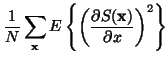
Now, each sample point in the 4D field is a random variable, with expectation given by equation 30. Therefore, due to the linearity of the expectation, the results can be averaged over all the sample points to achieve a more accurate estimate. That is, for a single point in time only:

$$\lambda_{11} = \frac{1}{N} \sum_{\ensuremath{\mathbf{x}}} ... ...rac{\partial S(\ensuremath{\mathbf{x}})}{\partial x} \right)^2$$ (33)

such that

$$E\{ \lambda_{11} \} = \frac{1}{N} \sum_{\ensuremath{\mathbf{x}}} E\left\{ \left( \frac{\partial S(\ensuremath{\mathbf{x}})}{\partial x} \right)^2 \right\}$$ (34)

$$= \frac{1}{N} \sum_{\ensuremath{\mathbf{x}}} \frac{1}{2 {\sigma_x}^2}$$ (35)

$$= \frac{1}{2 {\sigma_x}^2}.$$ (36)

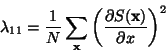Similarly for $\lambda_{22}$ and $\lambda_{33}$.

Note that $E\{ \lambda_{11} \} = \frac{1}{2 {\sigma_x}^2}$, $E\{ \lambda_{22} \} = \frac{1}{2 {\sigma_y}^2}$ and $E\{ \lambda_{33} \} = \frac{1}{2 {\sigma_z}^2}$ is the same notation used in [2].