In order to calculate the average group activation, we model the individual subject activation as being normally distributed according to
where
![]() represents the average group activation and is usually estimated as
represents the average group activation and is usually estimated as
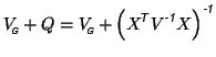
We will model the first-level within-subject covariances to be subject-specific and model the between-subject variances (from the group mean) as equal across the group. That is
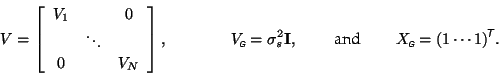
Then the adjusted second-level covariance matrix is
 |
|||
![\begin{displaymath}\left[
\begin{array}{ccc}
\left(X_1^{\mbox{\scriptsize\textit...
...{\sffamily {-1}}}}
\end{array} \right]+\sigma_s^2{\mathbf {I}}.\end{displaymath}](img112.png) |
Define
![]() , which is the sum of the within- and between-subject covariances.
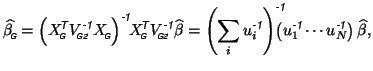
Then the estimate of the group parameter writes as
, which is the sum of the within- and between-subject covariances.
Then the estimate of the group parameter writes as
Hence we see that in the general framework, the mean group
activation parameter is a weighted average of the combined subject-
specific activations, where the weights are inversely proportional
to the subject-specific variances.
This adjustment is advantageous in the case where
the individual time-series model does not fit well for a particular
subject, ![]() , generating an unusual value for
, generating an unusual value for
![]() (an
outlier) but also a large
(an
outlier) but also a large
![]() . If no correction
for the first-level variance is done, then this outlier can
significantly affect the estimation of the group (between-subject)
variance. If, however, this first-level correction is performed, the
increased variance in this parameter will effectively de-weight the
contribution of this outlier to the group variance estimate, since we
use General Least Squares estimation.
. If no correction
for the first-level variance is done, then this outlier can
significantly affect the estimation of the group (between-subject)
variance. If, however, this first-level correction is performed, the
increased variance in this parameter will effectively de-weight the
contribution of this outlier to the group variance estimate, since we
use General Least Squares estimation.
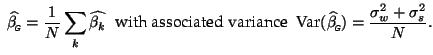
In the much simpler case, where the within-subject covariances are
![]() , and the
, and the ![]() are normalised, such that
are normalised, such that
![]() for all
for all ![]() , then
, then
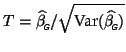
The test for significance is then carried out in a ![]() -test where
-test where