Numerical simulation

Figure 1: Expected % $Z$-score increase for the mean group activation for the case of typical first level covariance containing a few large outliers with different group sizes (N=6, 12 and 30). The first three images shows the increase as a function of the ratio of group level and mean first-level standard deviations ( $\sigma_{s}/ \langle\sigma_{k}\rangle$ on the $x$-axis) vs. relative group level activation ($y$-axis). Contour lines are shown for group-level $Z=2.0$ and $Z=3.0$ in the case of the heteroscedastic model (equation 16; solid lines) and the homoscedastic model (OLS; equation 17; dash-dotted). The difference between the solid and dash-dotted lines corresponds exactly to the color-coded percentage increase. The boxplots show the individual first level standard deviation compared to their mean ( $\sigma_{k}/\langle\sigma_{k}\rangle$) as an indicator of heteroscedacity. The percentage changes, which are independent of $\beta_{\mbox{\tiny\textit{\sffamily {$\!$G}}}}^{\mbox{}}$, are summarised in the fourth plot for all three variance configurations.

In this section we illustrate the potential benefit of a heteroscedastic variance model (i.e. by allowing for separate first-level variances) compared to the homoscedastic variance model (otherwise known as OLS for random-effects analysis of FMRI data [9]).

Both the heteroscedastic model (equation 16) and the homoscedastic model (equation 17) provide an unbiased estimate of the group level parameter of interest $\beta_{\mbox{\tiny\textit{\sffamily {$\!$G}}}}^{\mbox{}}$. They differ, however, in their associated variance, $\textrm{Var}(\widehat{\beta_{\mbox{\tiny\textit{\sffamily {$\!$G}}}}^{\mbox{}}})$, and therefore will give different $Z-$ or $T-$statistic. The associated variance for the heteroscedastic model is always less than or equal to that of the homoscedastic model, as can be shown using Jensen's inequality. This will result in an increase in the expected statistics values for the model in equation 16:

$$\frac{\langle\Delta Z\rangle}{\langle Z_{\mbox{\tiny homo}}\rangl... ...tiny\textit{\sffamily {$\!$G}}}}^{\mbox{}}})\rangle_{\mbox{\tiny hetero}}}}- 1$$

As a quantitative example of this increase we have generated a simulated group FMRI study, with a known set of first-level variances $V_k = \sigma_k^2{\mathbf {I}}$, together with a second-level variance $\sigma_s^2$. From these known values we calculate the expected percentage increase in $Z$- statistic (see above) and show this versus changes in the ratio of the second-level variance to the mean first-level variance (the assumed variance in the homo- scedastic model). First-level variances were taken from a real FMRI group study (simple motor paradigm) estimated using the GLS pre-whitening approach as implemented in FILM (part of FSL [7,17]). These estimates of first-level variances are realistic representatives of typical first-level variance structures and are defined to be ground-truth in the following simulation.

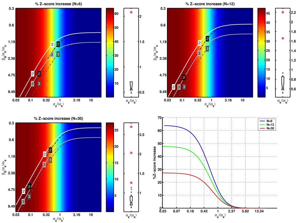
Figure 1 shows the expected percentage increase in $Z$-scores for three different sets of first-level variances, each of them containing one or more 'outliers' (see boxplots). As can be seen from the first three images, the expected percentage increase, for a given first-level variance structure, only depends on the ratio of second-level variance to mean first-level variance ( $\sigma_s/\langle\sigma_k\rangle$) and is independent of the group-level effect size $\beta_{\mbox{\tiny\textit{\sffamily {$\!$G}}}}^{\mbox{}}$. As the second- level variance becomes considerably larger than the mean first- level variance, the expected increase in $Z$-score tends to zero. When these variances are approximately equal, the heteroscedastic model allows for a $\sim 7 - 14\%$ increase in $Z$-score, increasing to much larger values as the second-level variance decreases relative to the mean first-level variance. The group-level effect size determines the actual $Z$-level, as shown by the overlaid contour plots (solid lines show $Z$- score levels for the heteroscedastic model while dash-dotted lines show the $Z$-score levels for the homoscedastic model). Over a large range of variance ratios the improvements gained by the heteroscedastic model have substantial implications on post- thresholded results, e.g. typical sub-threshold values of $2.0$ increase to super-threshold values of $\sim 3.0$.

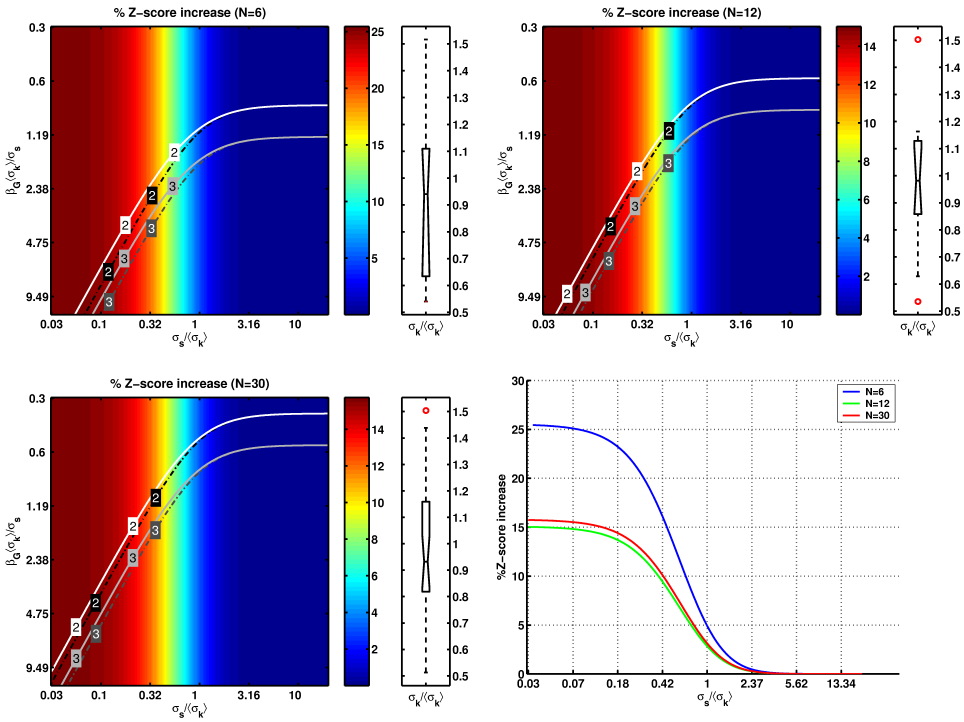
Figure 2 shows similar plots for cases where the first-level variances do not contain large outliers, that is, they are close to the homoscedastic model. In this case, the expected percentage $Z$-score increase is smaller, but still potentially important.

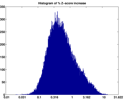
It is clear from these figures, that the exact configuration of first-level variances has a major impact on the improvements gained by using the heteroscedastic model. This dependency is further investigated in figure 3, where we show the expected (log-) increase in $Z$-score for a set of variance configurations estimated from $50200$ voxels in a real group study, assuming equal second-level and mean first-level variances. This histogram shows that approximately $1000$ voxels have a $> 5\%$ increase in expected $Z$-score.

Figure 2: Expected % $Z$-score increase for the mean group activation for the case of typical first level covariance (no large outliers) with different group sizes (N=6, 12 and 30). See figure 1 for details.

Figure 3: Histogram of log- % $Z$-score increase (50200 voxels, N=12 subjects, $\sigma_s/\langle\sigma_k\rangle=1$): $\sim 2$% of voxels (about 1000) have an increase of $>5$% in $Z$-score.