Methods

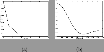
It turns out that the regressor used in the design matrix considerably affects the relative efficiency between colouring and prewhitening. To illustrate this we use a typical autocorrelation estimated for a grey-matter voxel (shown in figure 5) to give a typical $\mathbf{V}$ matrix, and use for $\mathbf{X}$ one of four different types of regressors of particular interest:

(a)

a boxcar design with period 60 secs

(b)

a single-event (SE) design with fixed inter-stimulus interval (ISI) of 15 secs and stimulus duration of 0.1 secs (Bandettini and Cox, 2000)

(c)

a single-event design with stimulus duration of 0.1 secs with jittering such that the ISIs are drawn from a uniform distribution U(13.5 secs, 16.5 secs)(Josephs et al., 1997)

(d)

a single-event design with randomized ISI taken from a normal distribution with mean $6secs$ and standard deviation $2secs$ with no ISI less than $2secs$ (Burock et al. (1998), Dale and Buckner (1997) and Dale (1999)) and stimulus duration of 0.1 secs.

All four designs are convolved with the same gamma HRF:

$$f_G(t;a, b)=\frac{b^a}{\Gamma(a)}t^{a-1}e^{-bt}$$ (19)

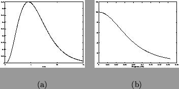
where the Gamma parameters $a,b$ are set according to mean $a/b=6 secs$ and variance $a/b^2=9{secs}^2$. The Gamma HRF for these parameters is shown in figure 6. More complicated HRF models could be used. However, any reasonable HRF model would be expected to have a similar spectral density and therefore behave in a similar way in this context. For all regressors TR is taken as 3 secs and all regressors have their means removed.

Figure 5: (a) Autocorrelation for a typical grey-matter voxel in a rest/null data set, and (b) the power spectral density for the same autocorrelation.

Figure 6: (a) Gamma HRF, $f_G(t;a, b)$ has parameters set according to mean $a/b=6 secs$ and variance $a/b^2=9{secs}^2$, and (b) the spectral density for the HRF.

The variance of the parameter estimates, $k_{\mbox{\scriptsize {\emph{eff}}}}\sigma^2$, is inversely proportional to the efficiency and can give us a measure of the relative efficiency of the different temporal filtering strategies. Although the estimation of $\sigma$ does depend upon the temporal filtering strategy used (equation 4 depends on $\mathbf{S}$), this effect is negligible. Subsequently, we define a measure of efficiency, $E$, relative to the maximally efficient prewhitening estimator for the regressor as:

$$E = \frac{k_{\mbox{\scriptsize {\emph{eff}}}} \mbox{ for prewhitening}} {k_{\mbox{\scriptsize {\emph{eff}}}}}$$ (20)

This was computed for each regressor using each of the three different temporal filtering strategies using equations 6, 7, 8 accordingly (there is only one regressor in each case so we use $c=[1]$). The low pass filter used for the colouring was matched to the HRF (figure 6). The values of $E$ for the randomised ISI and jittered ISI designs were averaged over $100$ randomly generated designs.