|
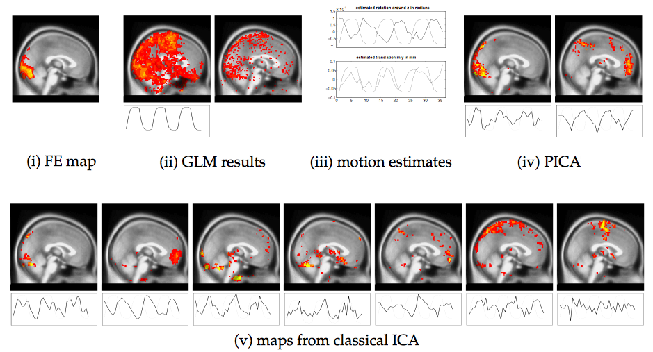
Figure 8(i) show the results from a fixed effects analysis over the
31 non-confounded data sets after each set was analysed separately
using FEAT. It shows the general visual activation pattern that emerged
from the analysis of sessions that were not heavily confounded by
subject motion. In contrast, figure 8(ii) shows
sagittal maximum intensity projections of ![]() score maps from a GLM
regression of one of the confounded data sets against the expected
response. There are large amounts of non-plausible and 'spurious'
activation. These results were obtained after initial rigid-body
motion correction using MCFLIRT. Visual inspection of the data after
correction suggested that the algorithm was able to realign the
volumes reasonably well with no 'noticable' misalignment of
neighbouring volumes. The estimated motion parameters in
figure 8(iii) suggest that the poor localisation of
visual cortical areas in the
score maps from a GLM
regression of one of the confounded data sets against the expected
response. There are large amounts of non-plausible and 'spurious'
activation. These results were obtained after initial rigid-body
motion correction using MCFLIRT. Visual inspection of the data after
correction suggested that the algorithm was able to realign the
volumes reasonably well with no 'noticable' misalignment of
neighbouring volumes. The estimated motion parameters in
figure 8(iii) suggest that the poor localisation of
visual cortical areas in the ![]() maps is not due to high magnitude of
motion but instead is a result of a strong correlation between certain
motion parameters and the stimulus sequence (stimulus correlated
motion). Within the GLM framework, the classical approach is to
include the estimated motion parameters as nuisance regressors. In
this case, however, the GLM results do not improve and still do not
uniquely identify visual cortical areas (figure
8(ii), second map).
maps is not due to high magnitude of
motion but instead is a result of a strong correlation between certain
motion parameters and the stimulus sequence (stimulus correlated
motion). Within the GLM framework, the classical approach is to
include the estimated motion parameters as nuisance regressors. In
this case, however, the GLM results do not improve and still do not
uniquely identify visual cortical areas (figure
8(ii), second map).
In the case of a PICA analysis of the motion confounded data
set, only seven component maps remained after dimensionality reduction
of which only 2 maps have an associated time course where the highest
power is at the frequency of stimulus presentation (figure
8(iv)). The results from a probabilistic independent
component analysis clearly improve upon the GLM results in that the
first PICA map shows a clean and well localised area of activation
within the visual cortex similar to the area identified by the fixed
effects analysis while the second map has large values at
the intensity boundraries of the original EPI data and has an
associated time course with high correlation to the estimated
rotation around the Z-axis (iii, top).
In comparison, figure 8(v) shows the
result of a standard ICA decomposition, where the data was projected
onto the dominant 29 eigenvectors in order to retain ![]() of the
variability in the data. Using the same criterion for the selection of
maps as before, seven components emerge (here ordered with decreasing
absolute correlation from left to right after thresholding by
converting each intensity value into a
of the
variability in the data. Using the same criterion for the selection of
maps as before, seven components emerge (here ordered with decreasing
absolute correlation from left to right after thresholding by
converting each intensity value into a ![]() score and only retaining
voxels with
score and only retaining
voxels with ![]() ). It is difficult to assess the differences
between figure 8(iv) and
(v) with respect to estimated motion. For the visual activation,
however,
the comparison suggests that results from classical ICA do actually
overfit the data in that different features that appear both in the
PICA map and fixed effects map are distributed across different
spatial maps.
). It is difficult to assess the differences
between figure 8(iv) and
(v) with respect to estimated motion. For the visual activation,
however,
the comparison suggests that results from classical ICA do actually
overfit the data in that different features that appear both in the
PICA map and fixed effects map are distributed across different
spatial maps.
|
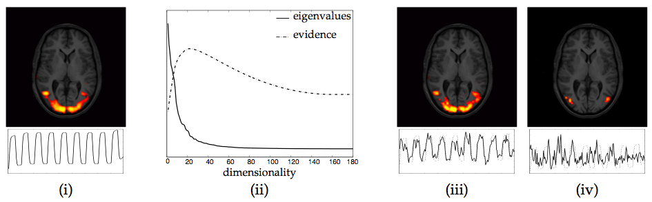
As a second example, figure 9 shows the PICA results
on the visual stimulation study used within the introduction to
illustrate the problem of overfitting. Based on the estimate of the
model order, the data was projected onto the first 27 eigenvectors
prior to the unmixing. Comparing figure 9(i) and (ii)
we get a much better correspondence between the areas of activation
estimated from the GLM approach and the main PICA estimate (compared
to figure
1(ii)). This is reassuring, since simple visual
experiments of this kind are known to activate large visual cortical
areas which should be reliably identifiable over a whole range of
analysis techniques. Within the set of IC maps a second source
estimate has an associated time course that correlates with the
assumed response at ![]() . This map depicts a bilateral pattern of
activation within visual cortical areas, possibly V3/MT, areas known
to be involved in the processing of visual motion. This is highly
plausible given that under the stimulation condition the volunteer was
presented with a checkerboard reversing at 8Hz. The associated time
course is very similar to the time course associated with the spatial
map (iv) in figure 1, but in the case of standard ICA,
only a unilateral activation is identified. This is not attributable
to the difference in the thresholding itself; the raw IC map in figure
1 does not allow for a bilateral activation pattern.
Instead, it turns out to be direct consequence of the existence of a
noise model: the standard deviation of the residual noise in the PICA
decomposition is comparably small within these areas. After
transforming the raw IC estimates
. This map depicts a bilateral pattern of
activation within visual cortical areas, possibly V3/MT, areas known
to be involved in the processing of visual motion. This is highly
plausible given that under the stimulation condition the volunteer was
presented with a checkerboard reversing at 8Hz. The associated time
course is very similar to the time course associated with the spatial
map (iv) in figure 1, but in the case of standard ICA,
only a unilateral activation is identified. This is not attributable
to the difference in the thresholding itself; the raw IC map in figure
1 does not allow for a bilateral activation pattern.
Instead, it turns out to be direct consequence of the existence of a
noise model: the standard deviation of the residual noise in the PICA
decomposition is comparably small within these areas. After
transforming the raw IC estimates
![]()
![]() into
into ![]() -scores, the well
localised areas emerge. In addition, figure
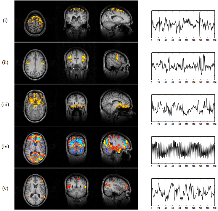
10 shows a selection of maps found during
the same PICA decomposition on this data, depicting e.g.
physiological 'noise', motion and scanner artefacts.
Note that in both examples the PICA maps are actual
-scores, the well
localised areas emerge. In addition, figure
10 shows a selection of maps found during
the same PICA decomposition on this data, depicting e.g.
physiological 'noise', motion and scanner artefacts.
Note that in both examples the PICA maps are actual ![]() statistical
maps and as such are much easier to compare against output from a
standard GLM analysis. Standard ICA maps, for reasons outlined above,
are simply raw parameter estimates and as such purely descriptive.
statistical
maps and as such are much easier to compare against output from a
standard GLM analysis. Standard ICA maps, for reasons outlined above,
are simply raw parameter estimates and as such purely descriptive.
|