Incorporation of prior knowledge

Within the framework of the standard GLM, spatial and temporal information like the assumed spatial smoothness of the areas of activation or temporal autocorrelation is incorporated into the modelling process by temporal and/or spatial filtering of the data prior to model fitting, e.g. the temporal characteristic of the hæ modynamic response is commonly encoded via the assumed and normally fixed convolution kernel.

The spatial and temporal filtering steps can also be used for data pre-processing for ICA. In the case of spatial smoothing note that since the inferential steps (see section 4 below) are not based on Gaussian Random Field theory [Worsley et al., 1996], we have the additional freedom of choosing more sophisticated smoothing techniques that do not simply convolve the data using a Gaussian kernel. Non-linear smoothing like the SUSAN filter [Smith and Brady, 1997] allow for the reduction of noise whilst preserving the underlying spatial structure and as a consequence reduce the commonly observed effect of estimated spatial pattern of activation 'bleeding' into non-plausible anatomical structure like CSF or white matter.

In the temporal domain, temporal highpass filtering is of importance since in FMRI low frequency drifts are commonly observed which can significantly contribute to the overall variance of an individual voxels' time course. If these temporal drifts are not removed, they will be reflected in the low-frequency part of the eigenvectors of the covariance matrix of the observations $R$$_{\mbox{\protect\boldmath $x$}}$ and increase the estimate for the rank of $A$. If the spatial variation between voxels' time courses is low, these areas of variability can be estimated as a separate source, e.g. B  $_0$ signal field inhomogeneities. If, however, the low frequency variations are substantially different between voxels, these effects ought to be removed prior to the analysis. For the experiments presented in this paper, we used linear highpass temporal filtering via Gaussian-weighted least squares straight line fitting [Marchini and Ripley, 2000].

In addition to these data pre-processing steps note that the estimates for the mixing matrix and the sources (equation 5) involve the estimate of the eigenvectors $U$ and the eigenspectrum $\Lambda$ of the data covariance matrix    $R$$_{\mbox{\protect\boldmath $x$}}=\sum_iw_i(\mbox{\protect\boldmath $x$}_i-\bar{... ...r{\mbox{\protect\boldmath $x$}})^{{\mbox{\scriptsize\textit{\sffamily {t}}}}},$ where $w_i$ is the contribution of voxel $i$'s time course to the covariance matrix. Typically, $w_i=\frac{1}{N} \quad \forall i$. In the case where prior information on the importance of individual voxels is available, we can simple encode this by choosing $w_i$ appropriately. As an example consider the case where we have results from an image segmentation into tissue types available: if $p$ is a vector where the individual entries $p_i$ denote the estimated probability of voxel $i$ being within gray-matter we can choose $w_i=p_i$ and the covariance is weighted by the probability of gray-matter membership. Simple approaches to performing ICA on the cortical surface (e.g. [Formisano et al., 2001]) are special cases of this, binarising $p$ and therefore losing valuable partial volume information. In this more general setting, however, the uncertainty in the segmentation will also be incorporated.

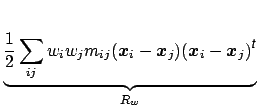
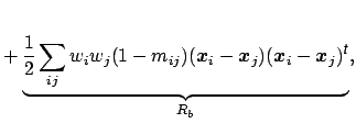
In order to incorporate more complex spatial information note that we can rewrite $R$$_{\mbox{\protect\boldmath $x$}}$ in the following form:

$$\mbox{\protect\boldmath$R$} _{\mbox{\protect\boldmath$x$}} = \underbrace{\frac{1}{2}\sum_{ij}w_iw_jm_{ij}(\mbox{\protect\boldm... ...ox{\protect\boldmath$x$}_j)^{{\mbox{\scriptsize\textit{\sffamily {t}}}}}}_{R_w}$$ (14)

$$+ \underbrace{\frac{1}{2}\sum_{ij}w_iw_j(1-m_{ij})(\mbox{\protect... ...{\protect\boldmath$x$}_j)^{{\mbox{\scriptsize\textit{\sffamily {t}}}}}}_{R_ b},$$

i.e. the canonical covariance matrix can be split into within-group and between-group covariance terms. The matrix $M$$=(m_{ij}); m_{ij}\in [0,1]$ defines a weighted graph of $N$ nodes and can encode any possible association between any pair of voxels that we want to introduce into the estimation. We can restrict calculation to the first term in equation 14 and perform the eigenvalue analysis on only the part of the covariance matrix generated by voxel pairs we believe to be associated with each other. In its general form the matrix $M$ has $N^2$ entries which for typical FMRI data sets requires vast amounts of memory. Often, however, the matrix $M$ can be sparse only having ${\cal O}(N)$ non-zero entries whilst still encoding a variety of spatial models, e.g. we can constrain the calculation to voxel pairs within a certain neighbourhood of fixed size.

In addition to spatial information, assumptions on the nature of the time courses can be incorporated using regularized principal component analysis techniques [Ramsay and Silverman, 1997]. Instead of filtering the data, constraints can be imposed on the eigenvectors, e.g. constraints on the smoothness can be included by penalizing the roughness using the integrated square of the second derivative. Alternatively it is possible to penalize the diffusion in frequency space, i.e. impose the constraint that the eigenvectors have a sparse frequency representation.