Apodization of the Cost Functions

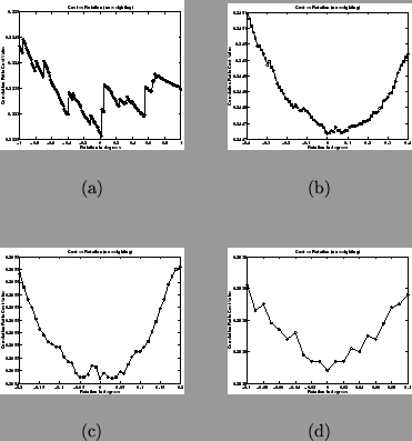
As seen in Figure 1, the local behaviour of the cost function shows small discontinuities as the transformation parameters are varied smoothly. This creates local minima ``traps'' for the optimisation method. Since all interpolation methods are continuous (except nearest neighbour which is consequently seldom used) the discontinuities are not due to the type of interpolation used. The cause of these discontinuities is the changing amount of overlap of the reference and floating image.

Figure 1: Plots of the Correlation Ratio cost function versus rotation about the $x$-axis, showing the presence of local discontinuities. Such discontinuities can sometimes signify the presence of local minima. The resolution of the images are: (a) 8mm, (b) 4mm, (c) 2mm and (d) 1mm. Note that the range of angles shown and the size of discontinuity decreases as the resolution scale decreases. Therefore the problem is greater at larger scales. Note that each individual sample of the cost function is denoted by a circle.

There are two different ways of treating values outside the Field of View (FOV) of an image:

1. Treat all values outside the FOV as zero.
2. Do all calculations strictly in the overlapping region.

The first method is undesirable as it creates artificial intensity boundaries when the object is not wholly contained within the FOV. However, in the second method the number of points counted in the overlapping region varies, not just the expressions involving intensities. Therefore, in the second case both the numerator and denominator of the cost functions (except Least Squares) will change discontinuously as the amount of overlap changes. The discontinuities exist because the images are discrete sets of voxels. In particular, the reference image defines a fixed set of voxel locations over which the cost function is calculated. Then, for a given transformation, the floating image intensities at these locations are calculated using interpolation. 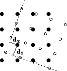A reference image voxel location is only counted when it is valid: that is, within the overlapping region such that it maps to a location inside the FOV of the floating image. When the edge of the FOV of the floating image crosses a reference voxel location, the location suddenly goes from being inside the overlapping region to outside, causing a discontinuous change in the number of valid locations, as shown in Figure 2.

Figure 2: Example showing how the overlapping region of the FOV for the reference image (filled dots) and floating image (open dots) can change with transformation. The shortest distances, $d_X$ and $d_Y$, (shown as a solid lines) to the edges of the overlapping region (shown by the dashed lines) are illustrated for a single reference voxel location.

We aim to apodize the cost function by removing these discontinuities. To do this, our approach has been to introduce a geometric apodization that de-weights the contributions of locations that are near the edge of the overlapping region. The weighting is chosen so that the contribution of such locations drops continuously until it reaches zero at the edge of the overlapping region. Any continuous weighting function could be used but for simplicity and computational efficiency we choose one that is linear. For instance, consider a 2D example of a reference location that maps to a point inside the overlapping region, where the distance from the nearest edges of the floating image FOV are $d_X$ and $d_Y$ units, as shown in Figure 2. In each dimension, if this value is less than some threshold $D$, then the influence of that point is weighted by a weight $w = d/D$. In higher dimensions, the product of the weighting functions in each dimension is used. That is: $w(d_X,d_Y,d_Z) = w(d_X) w(d_Y) w(d_Z)$. The weighting is applied to all terms involving that location's intensity as well as to the number of locations in the region. For example, consider the $n$th moment of an iso-set:

$$M_n\{Y_k\} = \frac{1}{N_k} \sum_{j \vert X_j \in I_k} (Y_j)^n$$ (2)

$$N_k = \sum_{j \vert X_j \in I_k} 1.$$ (3)

where $M_n$ is the $n$th moment, $j$ is a voxel index, $X$ and $Y$ represent the reference and floating images respectively and $I_k$ denotes the $k$th intensity bin. With general weighting this becomes:

$$M_n\{Y_k\} = \frac{1}{N_k} \sum_{j \vert X_j \in I_k} w_j \; (Y_j)^n$$ (4)

$$N_k = \sum_{j \vert X_j \in I_k} w_j.$$ (5)

where $w_j$ is the weight of the location $j$, which is 0 outside the overlapping region, $d/D$ for $d<D$ or 1 for $d \ge D$ inside the overlapping region. This weighting scheme can be simply and efficiently applied to any of the non entropy-based cost functions (i.e. LS, NC, W and CR). It depends on one parameter -- the threshold distance $D$ -- which can be varied to increase the amount of apodization. When $D=0$ there is no apodization, whilst increasing $D$ creates smoother and smoother cost functions, although the cost function will be continuous for any non-zero value of $D$. 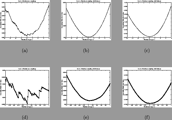Also note that making $D$ larger than the voxel spacing is permitted and just has a greater smoothing effect, as shown in Figure 3.

Figure 3: Plots of the Correlation Ratio cost function versus rotation at different values for the geometric apodization threshold, $D$. The values of $D$ shown are 0mm, 1mm and 8mm for the three columns (left to right respectively). The resolution in each case is 8mm and the bottom row shows the same values over an expanded scale. Each plot was generated by measuring the cost functions between two real images, about the estimate of the global minimum, which was a non-identity transformation and so did not correspond to maximum overlap of the FOVs. This clearly shows that the apodization has the desired smoothing effect on the cost function, eliminating large discontinuities. Note that each individual sample of the cost function in the bottom row is denoted by a circle.