Motion Correction

In broad terms, a motion correction algorithm must take a time series of fMRI images and register each image in the series to a reference image. This reference image may be of a different modality [1] but a more common approach is to select one image from the time-series itself (usually the first -- c.f. SPM [7]) and register the remaining images to this template image. If we make the reasonable assumption that there is unlikely to be large motion from one image to the next (usually 3 seconds between images or less), we can use the result of one image's registration as an initial guess for the next image in the series. This is accomplished by assuming an initial identity transformation between the middle image $V_{n}$ in a time series and the next adjacent image $V_{n+1}$ and then finding the optimal transformation $T_{1}$ by optimising the cost function. The resulting solution is then used as a starting point for the next optimisation with the next image pair $V_{n}, V_{n+2}$ (see Figure 6). This is only done at the lowest resolution, as all higher resolutions use the transformations found at the next lower resolution for the initial estimates.

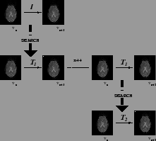
Figure 6: Schematic of the rigid-body motion correction scheme. The median indexed image of the series ($V_n$) is regarded as the reference image and each transformation ($T_1$) to an adjacent image is used as the initial `guess' for the transformation between that image and the one beyond ($V_{n+1}$; $n$++ signifies an increment of $n$).

The final schedule carries out the following steps on the uncorrected data (optional stages are shown in italics):

• 8mm optimisation using the middle image as initial reference and then using each result to initialise next pairwise optimisation
• 4mm optimisation using middle image as reference and 8mm stage results as initialisation parameters
• 4mm optimisation (lower tolerance) using middle image as reference and 4mm stage results as initialisation parameters
• Mean Registration option:
  • Apply transformation parameters from high tolerance 4mm stage
  • Average corrected images to generate mean template image
  • Carry out 8mm, 4mm and 4mm (high tolerance) optimisations as before but against mean image as reference.
• Sinc Registration option:
  • Carry out additional 4mm (high tolerance) optimisation using sinc interpolation (instead of trilinear as used in previous stages)
• Apply current transformation parameters to uncorrected data and save