Cost Function

Many different cost functions have been proposed for image registration problems. Some use geometrically defined features, found within the image, to quantify the (dis)similarity, whilst others work directly with the intensity values in the images. A large comparative study of different registration methods [17] indicated that intensity-based cost functions are more accurate and reliable than the geometrically-based ones. Consequently, most recent registration methods have used intensity-based cost functions, and these are the ones which will be discussed in this paper. Intensity-based cost functions can be divided naturally into two categories: those suitable for intra-modal problems and those suitable for inter-modal problems. In the former category the most commonly used cost functions are: least squares (LS) and normalised correlation (NC). 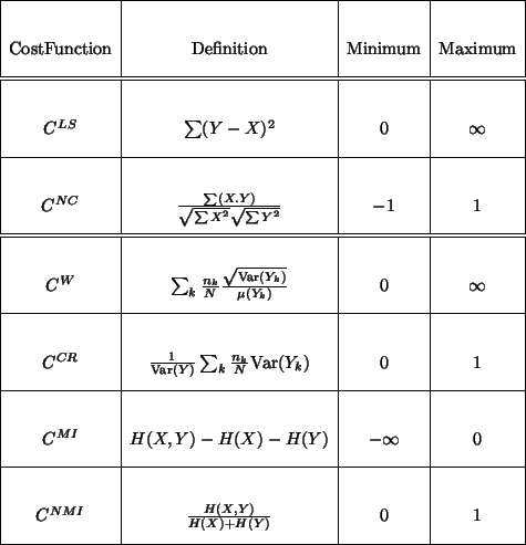For the latter, and more difficult, category the most commonly used functions are: mutual information (MI), normalised mutual information (NMI), woods (W) and correlation ratio (CR). These functions are defined mathematically in Table 1 (see [12] for more information).

Table 1: Mathematical definitions of the most commonly used intensity-based cost functions: Least Squares (LS); Normalised Correlation (NC); Woods (W); Correlation Ratio (CR); Mutual Information (MI); and Normalised Mutual Information (NMI). The notation is: quantities $X$ and $Y$ denote images, each represented as a set of intensities; $\mu (A)$ is the mean of set $A$; $\ensuremath{{\mathrm{Var}}}(A)$ is the variance of the set $A$; $Y_k$ is the $k$th iso-set defined as the set of intensities in image $Y$ at positions where the intensity in $X$ is in the $k$th intensity bin; $n_k$ is the number of elements in the set $Y_k$ such that $N = \sum_k n_k$; $H(X,Y) = - \sum_{ij} p_{ij} \log p_{ij}$ is the standard entropy definition where $p_{ij}$ represents the probability estimated using the $(i,j)$ joint histogram bin, and similarly for the marginals, $H(X)$ and $H(Y)$. Note that the sums in the first two rows are taken over all corresponding voxels.