Relating Fully Bayesian Inference to Frequentist Inference

We have a number of choices for how we use the posterior distribution $p(c^T\beta_g\vert Y)$. We could simply use the posterior, $p(c^T\beta_g\vert Y)$, to build up posterior probability maps representing the probability of activation at each voxel (10). Another possibility is the use of (spatial) mixture modelling (14,23,6) to classify voxels as activating and non-activating. We do not attempt to explore or discuss the relative merits of these approaches in this paper. Here, we consider another possibility of the inference produced if we mimic null-hypothesis frequentist inference (i.e. controlling a False Positive Rate (FPR)) by assuming that under the null hypothesis the z-statistics, that the fully Bayesian [BIDET] approach produces, are standardised (zero mean and standard deviation of one) Normally distributed.

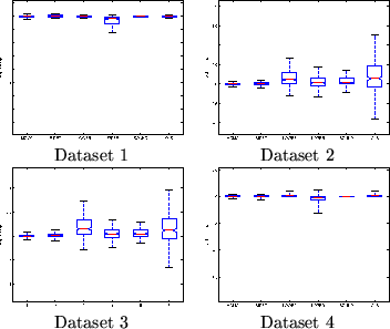
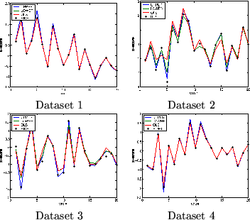
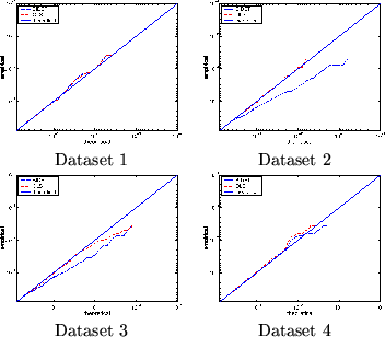
To examine this possibility, figure 6 shows the log probability-log probability plots for the four different datasets for [BIDET] and [OLS]. These are plots of the nominal/theoretical frequentist FPR against the probabilities obtained empirically from our four null artificial datasets. For all four datasets [OLS] does, as expected, produce a log probability plot that matches the nominal/theoretical frequentist FPR. However, this is not true for the [BIDET] approach.

Datasets 1 and 4 with small $\sigma_{\beta_k}$ compared to $\sigma_g$ gives close to the same inference using [BIDET] as when using [OLS]. Hence, we would expect the log probability that [BIDET] produces to match the nominal/theoretical frequentist FPR. Figure 6 demonstrates that this is true.

However, for Datasets 2 and 3 ( $\sigma_{\beta_k}^2$ is of the same order as $\sigma_g$) [BIDET] produces different results to [OLS]. The empirical log probabilities are lower than the nominal/theoretical FPR in figure 6(b) and (c). Recall from section 6.1.3, that we have two ways in which we expect z-statistics to change between [OLS] and [MCMC]. Firstly, they can increase due to increased efficiency from using lower-level variance heterogeneity. Secondly, they can decrease due to the higher-level variance being constrained to be positive. The first of these effects will introduce no bias into the p-p plots. Hence, only the second of these effects will be visible and the p-p plots for datasets 2 and 3 in figure 6 are consistent with this.

This means that whilst we produce more accurate estimates of the total mixed effects variance, it also means that the z-statistics resulting from [BIDET] are not standardised Normally distributed under the null hypothesis. This is not a problem if we just report posterior probability maps or use mixture modelling.

However, if we do choose to proceed with assuming that the z-statistics from [BIDET] are standardised Normally distributed, since the empirical log probabilities are lower than the nominal/theoretical frequentist FPR, then the validity of our statistics will not be violated. In other words, the z-statistics from [BIDET] are, on average conservative. The disadvantage of this is that we will lose some sensitivity when compared with using the unknown, correct null distribution. The advantage is that we can utilise cluster based inference techniques on the z-statistic maps, such as Gaussian Random Field Theory (21,26).

Figure 2: Boxplots over 400 voxels showing the z-statistics obtained from a long MCMC chain of 200,000 samples minus the z-statistics obtained from the different inference approaches considered. The box has lines at the lower quartile, median, and upper quartile values. The length of the whiskers is 1.5 times the Inter Quartile Range. The boxplots labelled [MCMC] correspond to the difference in z-statistics between those obtained from the 200,000 sample MCMC chain and those obtained from another 200,000 sample MCMC chain with a different random seed. The boxplots labelled [BOUND] correspond to how far outside the fast approximation bound (described as [UPPER] and [LOWER]) the z-statistics obtained from the 200,000 sample MCMC chain are.

Figure 3: Plots showing the z-statistics for 20 voxels obtained from different inference approaches for the 3 different artificial datasets.

Figure 4: Histograms over 400 voxels of the DOF estimated by [BIDET] for the different datasets for the 3 different artificial datasets.

Figure 5: Boxplots over 400 voxels showing the difference in z-statistics between those obtained from a long MCMC chain of 200,000 samples and those obtained from using BIDET on MCMC chains of varying sample sizes on Dataset 1. The box has lines at the lower quartile, median, and upper quartile values. The length of the whiskers is 1.5 times the Inter Quartile Range.

Figure 6: Log probability-log probability plots over 400 voxels for the four different datasets for [BIDET] and [OLS]. These show plots of (nominal/theoretical) FPR against that obtained experimentally from our 3 null artificial datasets. The straight diagonal line shows the result for what would be a perfect match.