In this section we describe how the multivariate non-central t-distribution fit is performed in BIDET.
Assume that we have
![]() matrix,
matrix, ![]() , with elements,
, with elements,
![]() , where
, where
![]() indexes samples and
indexes samples and
![]() indexes parameters. The task is to fit to these samples a
multivariate non-central t-distribution,
indexes parameters. The task is to fit to these samples a
multivariate non-central t-distribution,
![]() (as described in appendix 10.3).
(as described in appendix 10.3).
In BIDET we constrain the mean of the multivariate non-central
t-distribution,
![]() , to be equal to that from the fast
posterior approximation for
, to be equal to that from the fast
posterior approximation for
![]() described in
section 3.5. If we are not using this constraint
then we can set the mean
described in
section 3.5. If we are not using this constraint
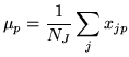
then we can set the mean ![]() to the sample mean, i.e:
to the sample mean, i.e:
 |
(27) |
| (28) |
We still need to estimate ![]() and
and ![]() . Fortunately, we
can represent a multivariate non-central t-distribution using a
two-parameter gamma distribution and a multivariate Normal
distribution in a Bayesian framework, by introducing hidden
variables
. Fortunately, we
can represent a multivariate non-central t-distribution using a
two-parameter gamma distribution and a multivariate Normal
distribution in a Bayesian framework, by introducing hidden
variables ![]() (see appendix 10.3). With hidden
variables we can use the Expection-Maximisation (EM) algorithm. In
the E-step we obtain the expected value of the hidden variables,
(see appendix 10.3). With hidden
variables we can use the Expection-Maximisation (EM) algorithm. In
the E-step we obtain the expected value of the hidden variables,
![]() :
:
 |
(29) |
| (30) |
 |
|||
| (31) |