


Next: Marginalising over in the
Up: Appendix
Previous: Multivariate Non-central t-distribution fit
Determining Reference Priors
Here we show how we determine the reference prior for a vector of
parameters  for a model with likelihood
 .
This is taken from section 5.4.5. of (2):
.
This is taken from section 5.4.5. of (2):
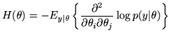
The Fisher information matrix,
 , is given by:
 |
|
|
(32) |
For the models in this paper, the Fisher information matrix,
, is block diagonal:
![$\displaystyle H(\vec{\theta}) \! =\! \left[\! \begin{array}{cccc}
h_{11}(\vec{\...
... 0 & \ddots & 0 \\
0 & \hdots & 0 & h_{mm}(\vec{\theta})
\end{array}\! \right]$](img228.png) |
|
|
(33) |
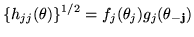
and we can separate out the block
 as being
the product:
as being
the product:
 |
|
|
(34) |
where
 is a function depending only on
  and
and
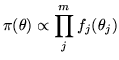
 does not depend on . The
Berger-Bernardo reference prior is then given by:
does not depend on . The
Berger-Bernardo reference prior is then given by:
 |
|
|
(35) |
Note that this approach yields the Jeffreys prior in
one-dimensional problems.
Next: Marginalising over in the
Up: Appendix
Previous: Multivariate Non-central t-distribution fit