


Next: Gradient of the Perturbed
Up: Theory
Previous: Case 3:
Due to the linearity of equation 18 the single voxel solutions
derived in the previous section can be added together to give the
total field for the object as
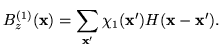 |
(24) |
This takes the form of a discrete convolution of the discrete
susceptibility map,  , and the single voxel solution,
  .
Therefore the calculation can be efficiently implemented by using the
3D Fast Fourier Transform (FFT) as
.
Therefore the calculation can be efficiently implemented by using the
3D Fast Fourier Transform (FFT) as
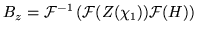 |
(25) |
where
 is the FFT and
  is a zero-padding
function, used to ensure that there is no period wrap-around in the
convolution.
is a zero-padding
function, used to ensure that there is no period wrap-around in the
convolution.