Basis Functions

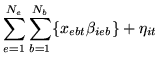
In this work we model the different HRF shapes for different underlying conditions at different voxels using basis functions and assuming a linear time invariant system (Josephs et al., 1997). If we have $e=1\ldots N_e$ underlying conditions, and for each condition we have $b=1\ldots N_b$ basis functions to model the HRF for that condition for voxel $i$ we can rewrite equation 1 as:

$$y_{it} = \sum_{e=1}^{N_e} \sum_{b=1}^{N_b} \{x_{ebt} \beta_{ieb}\} + \eta_{it}$$ (9)

where $\beta_{ieb}$ is the regression parameter for the $b^{th}$ basis function of the $e^{th}$ underlying condition at voxel $i$ and:

$$x_{eb\tau} = g_{b\tau }\otimes s_{e\tau}$$ (10)

where $\otimes$ represents convolution, $g_{b\tau}$ is the $b^{th}$ basis function and $s_{e\tau}$ is the $e^{th}$ stimulus function. Note that $\tau$ is an index at higher temporal resolution than $t$, to capture all of the HRF shape (i.e. for a resolution of $1/\rho$ of a TR, $\tau=1,\ldots,\rho T$). We obtain $x_{ebt}$ from $x_{eb \tau}$ by sampling every $\rho^{th}$ $x_{eb \tau}$.