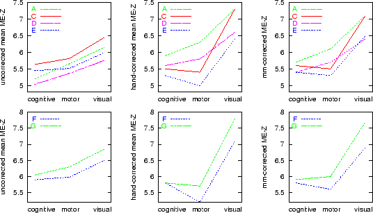
Mean ME-Z plots are shown in Figure 8. Higher ME-Z implies less analysis-induced inter-session variance, or, viewed another way, greater robustness to session effects.
Before discussing these plots it is instructive to get a feeling for
what constitutes ``significant'' difference in the plots. Suppose that
two ME-Z maps were, in these figures, separated by a Z difference of
0.25. This would correspond to a general relative scaling between the
two maps of approximately ![]() . We are interested in the
effect that this difference has on the final thresholded activation
map. Therefore we can estimate this effect by thresholding a ME-Z map
at a standard level and also at this level scaled by 4%. Thresholding
at
. We are interested in the
effect that this difference has on the final thresholded activation
map. Therefore we can estimate this effect by thresholding a ME-Z map
at a standard level and also at this level scaled by 4%. Thresholding
at ![]() , when corrected (using Gaussian random field theory) for
multiple comparisons, corresponds to a Z threshold of approximately 5.
We therefore thresholded the three ME-Z images from analysis F at
levels of
, when corrected (using Gaussian random field theory) for
multiple comparisons, corresponds to a Z threshold of approximately 5.
We therefore thresholded the three ME-Z images from analysis F at
levels of ![]() and
and ![]() . For the cognitive, motor and visual ME-Z
images, this resulted in reductions in supra-threshold voxel counts by
11%, 8% and 6% respectively. These are not small percentages; we
conclude that a difference in 0.25 between the various plots can be
considered to be ``significant'' in terms of the effect on the final
reported mixed-effects activation maps. (Note that these different
thresholdings were carried out with two threshold levels on the
same ME-Z image for each comparison, hence the previous criticism
of not comparing thresholded maps is not relevant here.)
. For the cognitive, motor and visual ME-Z
images, this resulted in reductions in supra-threshold voxel counts by
11%, 8% and 6% respectively. These are not small percentages; we
conclude that a difference in 0.25 between the various plots can be
considered to be ``significant'' in terms of the effect on the final
reported mixed-effects activation maps. (Note that these different
thresholdings were carried out with two threshold levels on the
same ME-Z image for each comparison, hence the previous criticism
of not comparing thresholded maps is not relevant here.)
We now consider plots A,C,D,E, the various tests which attempted to match all settings both to each other and to default usage. Firstly, consider comparisons which show the relative merits of the ``spatial'' components (motion correction and registration); A vs D and C vs E hold the statistics method constant whilst comparing spatial methods. Next, consider comparisons which show the relative merits of the statistical components (time-series analysis); A vs C and D vs E hold the spatial method constant whilst comparing statistical components. Finally, A vs E tests pure-FSL against pure-SPM.
Plots F and G test pure-SPM and pure-FSL respectively, with these analyses set up to match the specifications of the original analyses in [18], including turning on intensity normalisation in both cases.
The results show that both time-series statistics and spatial components (primarily head motion correction and registration to standard space) contribute to (i.e., add to) apparent session variability. Overall, with respect both to spatial alignment processing and time series statistics, FSL induced less error than SPM, i.e., was more efficient with respect to higher-level activation estimation.
The experiments used for this paper used a block-design, and as such are not expected to show up the increased estimation efficiency of prewhitening over precolouring [22]. In, [5], a similar study to that presented here, first-level statistics were obtained using SPM99 and FSL (i.e., only time-series statistics were compared, not different alignment methods). The data was primarily event-related, and, as in this paper, simple second-level mixed-effects analysis was used to compare efficiency of the different methods. The results showed that prewhitening was not just more efficient at first-level, but also gave rise to increased efficiency in the second-level analysis.