Flat Intensity Prior

Initially consider the case of a flat prior on $\alpha$. In this case let the range of each individual $\alpha$ be 0 to $L = C_1^{-1}$ such that, then $p(\alpha) = C_1^{D}$. When included, $\alpha$ parameters associated with linear intensity gradients have the appropriate columns of $G$ scaled so that the range of $\alpha$ is $-C_1^{-1}/2$ to $+C_1^{-1}/2$, and $p(\alpha) = C_1^{D}$ is still true. Note that $C_1$ is a constant for all $\alpha$, and represents the inverse intensity range.

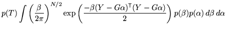
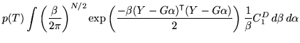
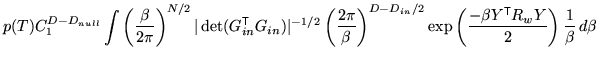
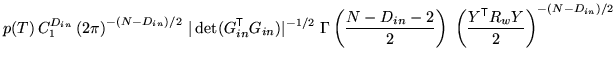
To start with, take the case where there are no uninteresting, degenerate or partial volume parameters. Note that there may be null parameters. In these conditions, the posterior can be simply calculated using the integrals in appendix A, giving

$$p(T\vert Y,S) \propto p(T) \int \left( \frac{\beta}{2 \pi} \right)^{N/2} \exp\left( \fr... ...{\textsf{T}}}(Y - G \alpha)}{2} \right) p(\beta) p(\alpha) \, d\beta \, d\alpha$$

$$\propto p(T) \int \left( \frac{\beta}{2 \pi} \right)^{N/2} \exp\left( \fr... ...tsf{T}}}(Y - G \alpha)}{2} \right) \frac{1}{\beta} C_1^{D} \, d\beta \, d\alpha$$

$$\propto p(T) C_1^D \int \left( \frac{\beta}{2 \pi} \right)^{N/2} \exp\lef... ...\alpha)}{2} \right) \frac{1}{\beta} \, d\beta \, d\alpha_{null} \, d\alpha_{in}$$

$$\propto p(T) C_1^D C_1^{-D_{null}} \int \left( \frac{\beta}{2 \pi} \right... ...f{T}}}(Y - G_{in} \alpha)}{2} \right) \frac{1}{\beta} \, d\beta \, d\alpha_{in}$$

$$\propto p(T) C_1^{D-D_{null}} \int \left( \frac{\beta}{2 \pi} \right)^{N/... ...\frac{-\beta Y^{\mathrm{\textsf{T}}}R_w Y}{2} \right) \frac{1}{\beta} \, d\beta$$

$$\propto p(T) C_1^{D_{in}} \left( 2 \pi \right)^{-(N-D_{in})/2} \vert\det(... ...)/2} \exp\left( \frac{-\beta Y^{\mathrm{\textsf{T}}}R_w Y}{2} \right) \, d\beta$$

$$\propto p(T) \, C_1^{D_{in}} \left( 2 \pi \right)^{-(N-D_{in})/2} \, \ver... ...ight) \; \left( \frac{ Y^{\mathrm{\textsf{T}}}R_w Y}{2} \right)^{-(N-D_{in})/2}$$

$$\propto p(T) \, C_1^{N} \, \vert\det(G_{in}^{\mathrm{\textsf{T}}}G_{in})\... ...\right) \; \left( C_1^2 \, Y^{\mathrm{\textsf{T}}}R_w Y \right)^{-(N-D_{in})/2}$$ (7)

where $D = D_{in} + D_{null}$, $\int_0^{L} d\alpha_{null} = L^{D_{null}} = C_1^{-D_{null}}$, $R_w = I - G_{in}( G_{in}^{\mathrm{\textsf{T}}} G_{in})^{-1} G_{in}^{\mathrm{\textsf{T}}}$, and $G_{in}$ is the submatrix formed from the $G$ matrix by only including columns associated with $\alpha_{in}$ parameters. That is, $G = [ G_{in} \; G_{null}]$ where $\alpha^{\mathrm{\textsf{T}}}= [ \alpha_{in}^{\mathrm{\textsf{T}}}\; \alpha_{null}^{\mathrm{\textsf{T}}}]$.

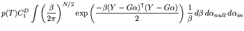
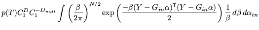
Note that $D_{in}$ and $G_{in}$ both depend on the transformation $T$. In fact, the dependence on $D_{in}$ is a form of normalisation for the number of degrees of freedom in the model. Also note that $D_{in} < N$ in all cases so that $N - D_{in} > 0$ and that increasing the normalised residuals $C_1^2 \, Y^{\mathrm{\textsf{T}}}R_w Y$ causes the posterior probability to decrease, as desired.

The above integrations use the approximation that

$$\int_0^L \exp\left( \frac{-\beta (Y - G \alpha)^{\mathrm{\textsf{... ...ta (Y - G \alpha)^{\mathrm{\textsf{T}}}(Y - G \alpha)}{2} \right) \, d\alpha_j$$

which is a good approximation when $\beta Y^{\mathrm{\textsf{T}}}G_j \gg 1$ and $\beta L G_j^{\mathrm{\textsf{T}}}G_j \gg 1$. This is true for $\alpha_j$ parameters where $G_j$ (the associated column of $G$) has a norm greater than 1.0 (i.e.  $G_j^{\mathrm{\textsf{T}}}G_j > 1$), and the true value of $\alpha$ is not within $1/\beta$ of the limits of the range (which can be easily ensured by slightly increasing the prior range). Note that $\beta Y_j^{\mathrm{\textsf{T}}}Y_j = SNR^2$, which is the squared Signal to Noise Ratio in voxel $j$ and typically much greater than 1.0 in MR images.

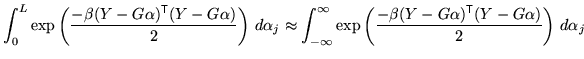
When these conditions are not true, the above approximation breaks down and the complimentary error function $\ensuremath{\mathrm{erfc}}$ terms, as shown in equation 14 in appendix A, must be included. This is true for pure partial volume parameters, and will be treated in section 3.2.2 which will be the last parameters to be integrated over.