Some parameters are associated only with a small partial volume
effect, normally at a single voxel, which can occur when a shape of
interest or the area of no interest partially overlaps a measured
voxel. The parameters will be called pure partial volume parameters,
![]() here. In this case the associated column of
here. In this case the associated column of ![]() has a
norm less than 1.0, and the finite range of
has a
norm less than 1.0, and the finite range of ![]() can no longer be
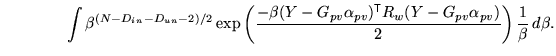
ignored. Hence the approximation of using equation 13
(in appendix A) must be replaced by the more accurate
integral of equation 14. However, in this case the
region of integration also becomes important. In the preceding
sections the variables are often transformed in order to compute the
integrals (the substitution
can no longer be
ignored. Hence the approximation of using equation 13
(in appendix A) must be replaced by the more accurate
integral of equation 14. However, in this case the
region of integration also becomes important. In the preceding
sections the variables are often transformed in order to compute the
integrals (the substitution ![]() which is done in
appendix A).
which is done in
appendix A).
For typical models, most columns of ![]() , apart from those associated
with
, apart from those associated
with
![]() , have norms that are much larger than 1.0, and are
almost orthogonal with the columns associated with these partial
volume parameters. Consequently, the effect of the change of
variables is to induce a slight rotation in the effective region of
integration. However, this effect is small and will be ignored here.
, have norms that are much larger than 1.0, and are
almost orthogonal with the columns associated with these partial
volume parameters. Consequently, the effect of the change of
variables is to induce a slight rotation in the effective region of
integration. However, this effect is small and will be ignored here.
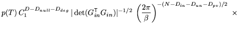
Applying the previous marginalisations of other ![]() parameters
first, leads to a posterior of the form
parameters
first, leads to a posterior of the form
 |
Using equation 14 and assuming that
![]() has negligible off-diagonal terms gives
has negligible off-diagonal terms gives
 |
|||
 |
|||
 |
(9) |
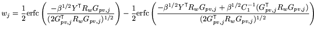
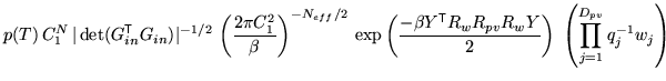
Note that it is now no longer possible to easily marginalise over
![]() as it appears in the complimentary error functions.
Consequently, the posterior has been left in the form
as it appears in the complimentary error functions.
Consequently, the posterior has been left in the form
![]() which can either be used with a pre-specified value of
which can either be used with a pre-specified value of ![]() (e.g. by estimating the SNR from the image) or numerically
marginalised.
(e.g. by estimating the SNR from the image) or numerically
marginalised.
Using the fact that
![]() and
and
![]() gives
gives
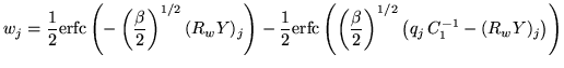
Furthermore, as
![]() then
then
![]() , and as
, and as
![]() then
then
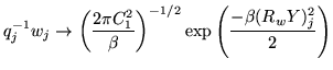
Also, as the partial volume overlap becomes small (
![]() )
then the posterior assumes the form that would result by increasing
)
then the posterior assumes the form that would result by increasing
![]() by 1 and including the residual intensity mismatch from
voxel
by 1 and including the residual intensity mismatch from
voxel ![]() back into the general residual term. This is what would
happen as this voxel makes the transition fully into the measured area
of interest, resulting in an extra effective voxel in the measurement
(the increase in
back into the general residual term. This is what would
happen as this voxel makes the transition fully into the measured area
of interest, resulting in an extra effective voxel in the measurement
(the increase in ![]() ) and the full inclusion of the residual
intensity error.
) and the full inclusion of the residual
intensity error.
In between these extreme values the contribution becomes partial. This can be compared to the form of de-weighting used for voxels at the edge of the valid field of view, in [3], which can be expressed in this notation as
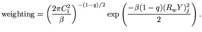
Note that the careful use of the finite range of ![]() and the
introduction of the complimentary error functions in the integrations
is crucial for making the posterior a continuous function of the
spatial transformation.
and the
introduction of the complimentary error functions in the integrations
is crucial for making the posterior a continuous function of the
spatial transformation.