Handling PTA-kmodes method

SAS/IML programs running with macro facilities have been written by the author to compute the SVD-kmodes of a tensor of any order [13] with or without non-identity metrics (R-functions are also available [14]). As stopping rule for the decomposition to finish, one can ask for a maximum number of k-modes solutions at each level of the algorithm, controlled by minimum amount of variability. Playing with these two sets of parameters allows either to get as close as wished to the full decomposition, or to pick up interesting Principal Tensors. Figure 1 shows what a PTA-3modes output listing looks like. The $3$-modes solutions are noted vs111, vs222, ... the associated $3$-modes solutions to the first mode (X) are noted Xvs11, Xvs22... One must notice that on the list of values the first associated solutions Xvs11 (or Yvs11, or Zvs11 ) are to be discarded in the decomposition as it is a repeat of vs111 because of the general algorithm: let $sx_1, sy_1, sz_1$ the first solution (i.e. $X..(sx_1 \otimes sy_1 \otimes sz_1)=vs111$, the solutions associated to $sx_1$ are obtained by the SVD-2modes of $X..sx_1$, therefore one finds again vs111 as the first singular values with solutions $sy_1, sz_1$. Nonetheless it is interesting to keep these repetitions because of the information given by the local decomposition (PCTloc: local percent of variability). PCT (respectively PCTloc) are in the percent of sum of squares (equal to percent of variance if the tensor is overall centred), then equals to the squared of the singular values divided by the total (local) sum of squares. In a PTA-$3$modes PCTloc refers to the usual percent of variability for an SVD; in general total refers to the original tensor analysed and local to the tensor currently decomposed i.e. associated solutions at a given level.

Figure 1: Example of output listing from PTA-3modes.

The notations are adapted for PTA-$k$modes (notations are slightly different with the R functions [14]), for example for a tensor of order 5:

1. $k$-modes solutions: vs11111, vs22222,...
2. associated $k$-modes first level: 1vs1111, 2vs1111..., 5vs1111, 1vs2222,...
3. associated $k$-modes second level: 1vs111,...,4vs666...,
4. associated $k$-modes third level: 1vs11,...,3vs66...

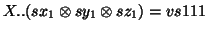
For each singular value, plots of components can then be produced using their normalised vector of coordinates. For the same Principal Tensor, plots of different components are read simultaneously as they correspond to the same singular value, but a basic rule must be kept to when interpreting the result. The sign of pairs of vectors are arbitrary, like in PCA, but unlike in PCA a solution is a triple of vectors (PTA-3modes) or a k-uple of vectors, then for example one has :

$$sx_1\otimes sy_1\otimes sz_1 =$$ (12)

$$(-sx_1)\otimes (-sy_1)\otimes sz_1=(-sx_1)\otimes sy_1\otimes (-sz_1)=sx_1\otimes (-sy_1)\otimes (-sz_1).$$

So one must read the associations or oppositions of items from different components (e.g. modalities, variables, spatial configuration) considering the product of the signs of their coordinates, i.e. once the principal tensor has been mentally rebuilt. Plots of the same component for different Principal Tensors can be produced but one must be aware of possible non-orthogonality when they are not both $k$-modes Principal Tensors (remember the decomposition is orthogonal on the whole space not ``completely" orthogonal in each space).