Extent of Minima

The number and location of local minima for a given cost function can only be determined empirically, as otherwise the registration problem could be solved analytically. However, the typical extent of local minima, the size of their basins of attraction and their inherent smoothness are important for designing effective optimisation strategies.

One approach for examining the cost function is to look at how it changes as individual parameter values vary about some fixed point. That is, to plot the function values versus one parameter value, with all other parameters held constant. This also avoids the problem of trying to visualise functions in high-dimensional spaces (for example, ${\mathcal R}^{12}$ for affine transformations).

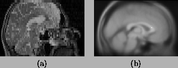
As it is the global minimum that is of most interest, the fixed point is chosen to be the global minimum itself. Figure 2 shows the cost function plots for each parameter (3 rotation angles, 3 translations, 3 scalings and 3 skews) using the images shown in figure 3. This image pairing was chosen as it had been found to be a difficult pair to register successfully. However, despite this fact, the global minimum is still quite broad and well defined.

  

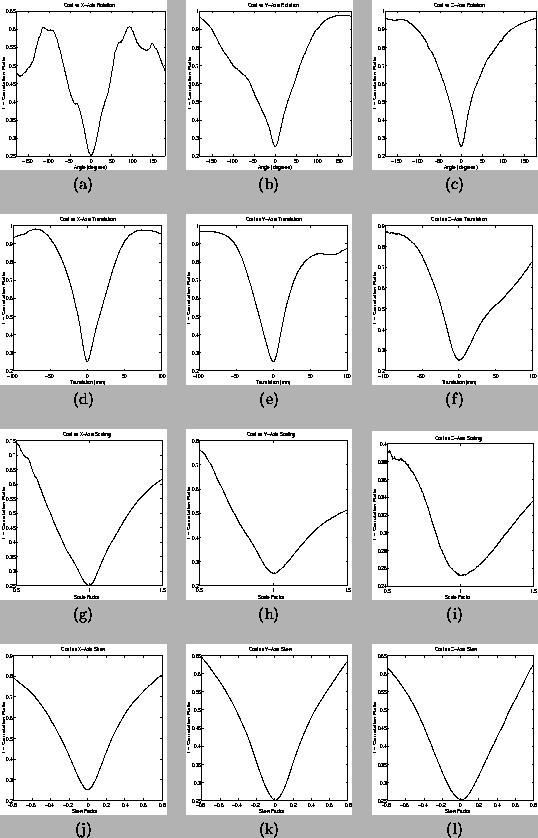
Figure 2: Plots of the Correlation Ratio cost function versus individual parameter values. In each plot, a single parameter is varied over a large range while the others are kept fixed. The central point about which the parameters varied was the global minimum. All cost function calculations were done using the image pair shown in figure 3 with a resampling (including appropriate pre-blurring) to cubic voxels with 8mm side-length.

  

Figure 3: Example slices from the volumes used for plotting the cost function. Figure (a) shows a T2 weighted image of a subject while figure (b) shows the MNI 305 image [Collins et al., 1994]. The voxel dimensions for these images were $0.93 \times 0.93 \times 5$ mm for (a), and $1 \times 1 \times 1$ mm for (b).

The plots shown in figure 2 give an idea of the gross behaviour of the cost function about the global minimum. However, on a small scale there exist many small, local minima, as shown in figure 4a. In addition, there also exist larger local minima as shown in figure 4b, where the central point is no longer the global minimum, but a transformation more typical of an initial alignment. Consequently a successful optimisation method must be able to cope with both small, densely packed local minima and much larger, and widely separated, local minima. These problems are respectively dealt with in section 4 by (1) an adaptive step local minimisation method (section 4.2) and (2) an initial search stage (section 4.3).

  

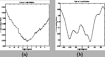
Figure 4: Plots of the cost function versus rotation about the x-axis, showing the presence of local minima. Figure (a) shows an expansion of the plot shown in figure 2a, over a small range about the global minimum. It can be seen that several small, local minima exist, generated by small fluctuations in the cost function. In figure (b) the cost function is plotted about a different central point -- one that is offset from the global minimum. This produces significant changes in the cost function, showing the presence of large local minima.