Non-spatial with Class Proportions

We can approximate the distribution in equation 5 by replacing the discrete labels, $x_i$, with continuous weights vectors, $\vec{w_i}$:

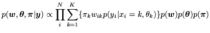$$p(\vec{w},\vec{\theta},\vec{\pi}\vert\vec{y}) \propto \prod_i^N \... ... \pi_k w_{ik}p(y_i\vert x_i=k,\theta_k)\} p(\vec{w})p(\vec{\theta})p(\vec{\pi})$$ (13)

where $\pi_k$ are the global class proportion parameters defined in equation 4 and represent the proportion of each class in the mixture model, and $p(\vec{w})$ is given by equations 10-12. Note that when we infer on the posterior, $\vec{\pi}$ will depend upon $\vec{w}$ in same way that $\vec{\pi}$ depends on $\vec{x}$ in the discrete labels mixture model.