Spatial

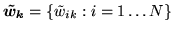
We can approximate the distribution in equation 8 by replacing the discrete labels, $x_i$, with continuous weights vectors, $\vec{w_i}$:

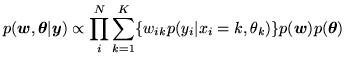$$p(\vec{w},\vec{\theta}\vert\vec{y}) \propto \prod_i^N \sum_{k=1}^K \{ w_{ik}p(y_i\vert x_i=k,\theta_k)\} p(\vec{w})p(\vec{\theta})$$ (14)

where $p(\vec{w})$, is given by equation 10 with $p(\vec{w}\vert\vec{\tilde{w}},\gamma) = \prod_i p(\vec{w_i}\vert\vec{\tilde{w}_i},\gamma)$ where as before $p(\vec{w_i}\vert\vec{\tilde{w}_i},\gamma)$ is specified by a deterministic mapping between $\vec{\tilde{w}}$ and $\vec{w}$ (the logistic transform, equation 12).

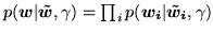
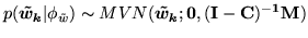
However, instead of equation 11, $p(\vec{\tilde{w}})$ is now a continuous Gaussian conditionally specified auto-regressive (CAR) or continuous MRF prior (Cressie, 1993) on each of the $K$ class maps, i.e. $p(\vec{\tilde{w}})=\prod_k p(\vec{\tilde{w}_k}\vert\phi_{\tilde{w}})$ (where $\vec{\tilde{w}}= \{ \vec{\tilde{w}_k}:k=1\ldots K$ } and $\vec{\tilde{w}_k}=\{\tilde{w}_{ik}:i=1\ldots N\}$) with:

$$p(\vec{\tilde{w}_k}\vert\phi_{\tilde{w}})\sim MVN(\vec{\tilde{w}_k};\mathbf{0},\mathbf{(I-C)^{-1}M})$$ (15)

where $\mathbf{C}$ is an ${N}\times {N}$ matrix whose (i,j)th element is $c_{ij}$, $\mathbf{M} = \frac{1}{\phi_{\tilde{w}}}\mathbf{I}$, and $\phi_{\tilde{w}}$ is the MRF control parameter which controls the amount of spatial regularisation. We set $c_{ii}=0$, $c_{ij}=1/N_{ij}$ if $i$ and $j$ are spatial neighbours and $c_{ij}=0$ otherwise (where $N_{ij}$ is the geometric mean of the number of neighbours for voxels $i$ and $j$) , giving approximately:

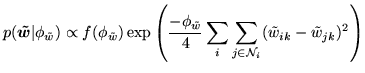$$p(\vec{\tilde{w}}\vert\phi_{\tilde{w}})\propto f(\phi_{\tilde{w}}... ...de{w}}}{4}\sum_i \sum_{j\in{\cal N}_i}(\tilde{w}_{ik}-\tilde{w}_{jk})^2 \right)$$ (16)

How does this posterior approximation using the continuous class weights vectors instead of class labels allow us to adaptively determine the amount of spatial regularisation? The answer is that $\tilde{w}_{ik}$ is a continuous random variable ranging effectively between $-\infty$ and $+\infty$ . Therefore, unlike $f(\phi_x)$ in equation 6, the normalising constant, $f(\phi_{\tilde{w}})$, in equation 16 is known:

$$f(\phi_{\tilde{w}})\propto \frac{1}{\phi_{\tilde{w}}^N}$$ (17)

and hence we can adaptively determine the MRF control parameter, $\phi_{\tilde{w}}$. To achieve this $\phi_{\tilde{w}}$ becomes a parameter in the model, and equation 14 becomes:

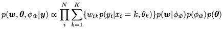$$p(\vec{w},\vec{\theta},\phi_{\tilde{w}}\vert\vec{y}) \propto \pro... ...k,\theta_k)\} p(\vec{w}\vert\phi_{\tilde{w}})p(\phi_{\tilde{w}})p(\vec{\theta})$$ (18)

where the prior $p(\phi_{\tilde{w}})$, is a non-informative conjugate gamma prior:

$$\phi_{\tilde{w}}\vert \tilde{a}_{{\tilde{w}}}, \tilde{b}_{{\tilde{w}}} \sim Ga(\phi_{\tilde{w}}; \tilde{a}_{{\tilde{w}}}, \tilde{b}_{{\tilde{w}}} )$$ (19)

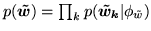
In summary, we have approximated the discrete labels with vectors of continuous weights which a priori approximate delta functions at 0 and 1. Each vector of continuous weights deterministically corresponds (via the logistic transform) to another vector of continuous weights, which a priori are uniform across the real line. As they are uniform across the real line these vectors of continuous weights can be regularised using a spatial prior (a continuous MRF) for which the amount of spatial regularisation can be determined adaptively.

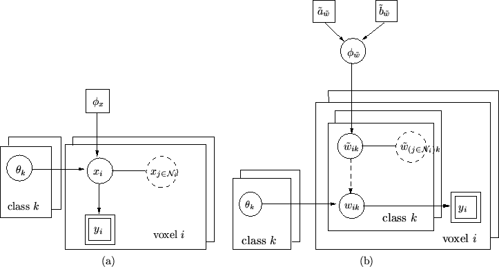
Figure 2 shows a graphical representation of the discrete labels mixture model (equation 8) and the continuous weights spatial mixture model with adaptive spatial regularisation (equation 14).

Figure 2: Graphical representation of (a) the discrete labels mixture model (equation 8), and (b) the continuous weights spatial mixture model with adaptive spatial regularisation (equation 14). Each parameter is a node in the graph and direct links correspond to direct dependencies. Solid links are probabilistic dependencies and dashed arrows show deterministic functional relationships. A rectangle denotes fixed quantities, a double rectangle indicates observed data, and circles represent all unknown quantities. Repetitive components are shown as stacked sheets. Dashed circles represent nodes that really correspond to a different stacked sheet, but which are shown on the top stacked sheet for ease of display.