Non-spatial without Class Proportions

We are going to approximate the distribution in equation 3 by replacing the discrete labels, $x_i$, with $K \times 1$ continuous weights vectors, $\vec{w_{i}}$:

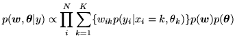$$p(\vec{w},\vec{\theta}\vert y) \propto \prod_i^N \sum_{k=1}^K \{w_{ik}p(y_i\vert x_i=k,\theta_k)\}p(\vec{w})p(\vec{\theta})$$ (9)

where $\vec{w}= \{ \vec{w_i}:i=1\ldots N$ } and $\vec{w_i}=\{w_{ik}:k=1\ldots K\}$ is the continuous weights vector at voxel $i$. Equation 9 only approximates equation 3 if we apply certain constraints to the continuous weights vectors. If we choose a prior on the continuous weights vector, $\vec{w_i}$, with the constraints that $0<w_{ik}<1$ and $\sum_k w_{ik}=1$, then as $p(\vec{w_i})$ tends to delta functions at $w_{ik}=0$ and $w_{ik}=1$, then equation 9 will tend to equation 3. Therefore, to apply these constraints the prior we use is:

$$p(\vec{w}) = p(\vec{w}\vert\vec{\tilde{w}},\gamma)p(\vec{\tilde{w}})$$ (10)

where:

$$p(\vec{\tilde{w}}) = \prod_{ik}^N p(\vec{\tilde{w}}_{ik})$$

$$p(\vec{\tilde{w}}_{ik}) = Uniform(\vec{\tilde{w}_{ik}};-\infty,+\infty)$$ (11)

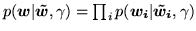and $p(\vec{w}\vert\vec{\tilde{w}},\gamma) = \prod_{i} p(\vec{w_i}\vert\vec{\tilde{w}_i},\gamma)$, where crucially $p(\vec{w_i}\vert\vec{\tilde{w}_i},\gamma)$ is a deterministic relationship by which $\vec{w_i}$ and $\vec{\tilde{w}_i}$ are related by the logistic transform:

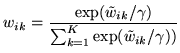$$w_{ik}=\frac{\exp(\tilde{w}_{ik}/ \gamma)}{\sum_{k=1}^K \exp(\tilde{w}_{ik}/ \gamma))}$$ (12)

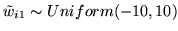
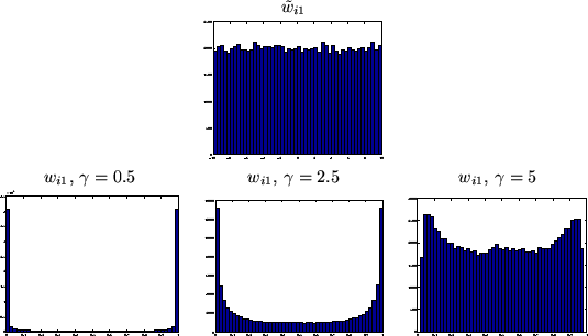
The normalising constant in the logistic transform ${\sum_{k=1}^K exp(\tilde{w}_{ik}/ \gamma)}$ ensures that the condition ${\sum_{k=1}^K w_{ik}=1}$ is met. This expression also ensures that $\tilde{w}_{ik}>\tilde{w}_{jk}$, if and only if $w_{ik}>w_{ij}$. Figure 1 shows how the logistic transform produces an approximation to the delta functions as $\gamma$ gets smaller. We fix the value of $\gamma$ to 0.05 whilst bounding $-10 < \tilde{w}_{ik} < 10$, this ensures that we get the desired approximation to delta functions at 0 and 1, whilst ensuring that we can compute $exp(\tilde{w}_{ik}/ \gamma)$ without causing overflow.

To summarise, we now have two vectors of continuous weights at each voxel, ${w}_{ik}$ and $\tilde{w}_{ik}$. $\tilde{w}_{ik}$ are weights which have a prior on them which is uniform on the real line. We then use the logistic transform to deterministically map the weights $\tilde{w}_{ik}$ to ${w}_{ik}$ at each voxel. Then, ${w}_{ik}$ are the continuous weights which represent approximations to the discrete labels with delta functions at 0 and 1.

Figure 1: Consider that we have the number of classes as $K=2$. [top] shows samples from the prior of $\tilde{w}_{i1}$, $\tilde{w}_{i1} \sim Uniform(-10,10)$ (samples from $\tilde{w}_{i2}$ are similar). [bottom] shows the samples from $w_{i1}$ ($w_{i2}$ is similar), which the samples from the prior of $\tilde{w}_{i1}$ and $\tilde{w}_{i2}$ transform to under the logistic transform with different values of $\gamma$ (equation 12). Hence, it can be seen how this produces a prior for $\vec{w_i}$, which approximates the desired delta functions at 0 and $1$ as $\gamma$ gets smaller.