


Next: Initialisation
Up: tr04mw2
Previous: Determining Basis Set Constraints
Inference
The distribution we are interested in inferring upon is the
posterior distribution
 (equation 3),
where
(equation 3),
where  is the set of parameters
 . It is not possible to solve for
this distribution analytically. Hence we use the framework
introduced to FMRI by Penny et al. (2003) of Variational Bayes. For a
general introduction to Variational Methods see Jordan (1999).
Using this approach we can approximate a posterior distribution
with
. It is not possible to solve for
this distribution analytically. Hence we use the framework
introduced to FMRI by Penny et al. (2003) of Variational Bayes. For a
general introduction to Variational Methods see Jordan (1999).
Using this approach we can approximate a posterior distribution
with
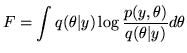
 by minimising the KL-divergence,
or equivalently by maximising the variational free energy,
by minimising the KL-divergence,
or equivalently by maximising the variational free energy,  ,
between them:
,
between them:
 |
|
|
(18) |
To maximise this function, we need to ensure that the resulting
integrals are tractable. A standard way to help achieve this is to
use conjugate priors and to factorise the approximate posterior.
In the modelling section, we parameterised the model in terms of
parameters  ,
,
 ,
,  and
and  , and wherever
possible specified conjugate priors on them. However, using these
parameters and factorising the posterior into
, and wherever
possible specified conjugate priors on them. However, using these
parameters and factorising the posterior into
 |
|
|
(19) |
is not tractable to Variational Bayes as we can not derive the
update equations for
 and
and
 . To
overcome this problem, instead of using the two parameters
. To
overcome this problem, instead of using the two parameters
 and
and
 , we reparameterise to use
 and
and
 by rewriting equation 11
as:
by rewriting equation 11
as:
where:
 |
|
|
(21) |
Recall from equation 11 that
 is the normalisation on the HRF shape vector,
, and the scalar,
, represents the size of
the HRF. We now have the following prior on
:
is the normalisation on the HRF shape vector,
, and the scalar,
, represents the size of
the HRF. We now have the following prior on
:
and a noninformative prior on
:
where the precision,
 , is fixed to be very
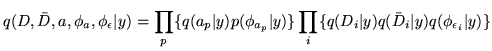
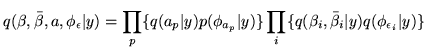
small (1e-6) for all voxels. We now assume the following
factorised form for the approximate posterior:
, is fixed to be very
small (1e-6) for all voxels. We now assume the following
factorised form for the approximate posterior:
 |
|
|
(24) |
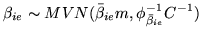
where:
where
 , where
  is the
 vector
![$ [ \beta_{i1} \hdots \beta_{ie} \hdots
\beta_{iN_e}]^T$](img163.png) and
and
 is the
 vector
![$ [ \bar{\beta}_{i1} \hdots \bar{\beta}_{ie} \hdots
\bar{\beta}_{iN_e}]^T$](img166.png) . Note that we do not fully factorise. We
would not expect
. Note that we do not fully factorise. We
would not expect  and
and
 to be independent a
posteriori. Therefore, we maintain a combined unfactorised
posterior for the two parameters and
.
However, we have factorised the noise parameter posteriors from
the regression parameter posteriors. This assumption helps to make
inference tractable using Variational Bayes. Penny et al. (2003)
discuss the implications of doing this and show that the error
induced by this assumption is negligible for inferring on FMRI
data. We also show later (in section 4) that there is
negligible error induced when inferring on artificial data.
At this point, the inference is still not fully tractable to
Variational Bayes as we can not derive the update equations for
to be independent a
posteriori. Therefore, we maintain a combined unfactorised
posterior for the two parameters and
.
However, we have factorised the noise parameter posteriors from
the regression parameter posteriors. This assumption helps to make
inference tractable using Variational Bayes. Penny et al. (2003)
discuss the implications of doing this and show that the error
induced by this assumption is negligible for inferring on FMRI
data. We also show later (in section 4) that there is
negligible error induced when inferring on artificial data.
At this point, the inference is still not fully tractable to
Variational Bayes as we can not derive the update equations for
 . To overcome this we rewrite the prior in
equation 22 as:
. To overcome this we rewrite the prior in
equation 22 as:
 |
|
|
(26) |
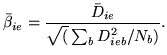
where the utility parameter,
 , is updated
as a point estimate equal to one over the current expected value
of
, is updated
as a point estimate equal to one over the current expected value
of
 :
:
where  is defined by the relationship
 , and
, and
 is the current marginal
covariance of
. The approximate posterior
distributions are now tractable to Variational Bayes. The update
rules for the approximate posterior distributions, which
iteratively maximises the free energy in
equation 18, are given in appendix B.
We can perform standard inference questions on the marginal
posterior over
is the current marginal
covariance of
. The approximate posterior
distributions are now tractable to Variational Bayes. The update
rules for the approximate posterior distributions, which
iteratively maximises the free energy in
equation 18, are given in appendix B.
We can perform standard inference questions on the marginal
posterior over  , in the same way that we do for the
standard use of basis functions in the GLM (i.e. using
f-contrasts, see section 3.2). We test the
accuracy of the posterior approximations presented in this section
using null artificial data in section 4.
The Variational Bayes inference requires approximately 10
iterations and takes approximately 15 minutes (for a whole brain -
in-plane resolution 4mm, slice thickness 7mm and
, in the same way that we do for the
standard use of basis functions in the GLM (i.e. using
f-contrasts, see section 3.2). We test the
accuracy of the posterior approximations presented in this section
using null artificial data in section 4.
The Variational Bayes inference requires approximately 10
iterations and takes approximately 15 minutes (for a whole brain -
in-plane resolution 4mm, slice thickness 7mm and  volumes) on
a 2GHz Intel PC.
volumes) on
a 2GHz Intel PC.
Subsections
Next: Initialisation
Up: tr04mw2
Previous: Determining Basis Set Constraints