Next: Artificial null data
Up: Inference
Previous: Initialisation
f-contrasts
Variational Bayes gives us an approximation to the posterior
distribution,
 . From this we can
obtain the approximate marginal posterior distribution,
. From this we can
obtain the approximate marginal posterior distribution,
 , as being a multivariate Normal
distribution (equation 25). If we write this as:
, as being a multivariate Normal
distribution (equation 25). If we write this as:
We can marginalise to get the marginal distribution over the
regression parameters,
 , as:
, as:
We can now use the marginal distribution in
equation 33 to perform inference. In this paper we
take the approach of using the f-contrast framework traditionally
used with basis functions in the frequentist GLM
framework (Josephs et al., 1997).
If  is a
is a
 vector representing an f-contrast,
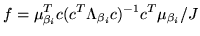
we can use the f-contrast framework to compute the normalised
power explained by the f-contrast:
vector representing an f-contrast,
we can use the f-contrast framework to compute the normalised
power explained by the f-contrast:
 |
|
|
(34) |
with degrees of freedom  and
and  . As with the use of basis
functions in the frequentist GLM framework (Josephs et al., 1997), we
lose directionality when doing an f-test. That is, we only
investigate the power explained by linear combinations of
the basis function parameters, regardless of the direction (i.e.
whether it is an activation or deactivation). This means that we
only look at the positive tail of the f-distribution to find both
activations and deactivations.
The alternative to doing a test on
. As with the use of basis
functions in the frequentist GLM framework (Josephs et al., 1997), we
lose directionality when doing an f-test. That is, we only
investigate the power explained by linear combinations of
the basis function parameters, regardless of the direction (i.e.
whether it is an activation or deactivation). This means that we
only look at the positive tail of the f-distribution to find both
activations and deactivations.
The alternative to doing a test on  would be to ask
``What is the probability that
would be to ask
``What is the probability that
 is greater than
zero?''. Recall from equation 11 that
, represents the HRF size (activation height). Can
we recover the activation height,
, from the
parameters we infer upon,
is greater than
zero?''. Recall from equation 11 that
, represents the HRF size (activation height). Can
we recover the activation height,
, from the
parameters we infer upon,
 and
and
 ? To
do this, we can rewrite equations 20 and
21 to get:
? To
do this, we can rewrite equations 20 and
21 to get:
Note that the term
 is the power we are testing when we do the f-test on
  .
Equation 35 tells us that we can use the sign of
to give the sign of
, and
therefore the direction of the activation.
We could look to derive the posterior probability of the
normalised power explained by the f-contrast in
equation 34. Instead, the approach we take in this paper
is to convert them to pseudo-z-statistics and then perform spatial
mixture modelling on the spatial map of pseudo-z-statistics as
described later. The f-to-z transform is carried out by doing an
f-to-p-to-z transform (i.e. by ensuring that the probabilities in
the tails are equal under the f- and z-distributions for the f-
and z-statistics).
We refer to them as pseudo-z-statistics as they are not
necessarily Normally distributed with zero mean and standard
deviation of one under the null hypothesis. This is because they
have been obtained by performing Bayesian inference. Whether or
not Bayesian inference produces the same null distribution as that
in frequentist inference will depend on the form of prior used. As
we shall see in section 4 and as we would
expect (Penny et al., 2003), if we use noninformative priors we do get
approximate equivalence between frequentist and Bayesian
inference. However, when we use constrained HRF shape priors we
get a different distribution under the null hypothesis. We will
see later how we can adjust to this different inference, and take
advantage of the extra sensitivity it offers, by using spatial
mixture modelling.
.
Equation 35 tells us that we can use the sign of
to give the sign of
, and
therefore the direction of the activation.
We could look to derive the posterior probability of the
normalised power explained by the f-contrast in
equation 34. Instead, the approach we take in this paper
is to convert them to pseudo-z-statistics and then perform spatial
mixture modelling on the spatial map of pseudo-z-statistics as
described later. The f-to-z transform is carried out by doing an
f-to-p-to-z transform (i.e. by ensuring that the probabilities in
the tails are equal under the f- and z-distributions for the f-
and z-statistics).
We refer to them as pseudo-z-statistics as they are not
necessarily Normally distributed with zero mean and standard
deviation of one under the null hypothesis. This is because they
have been obtained by performing Bayesian inference. Whether or
not Bayesian inference produces the same null distribution as that
in frequentist inference will depend on the form of prior used. As
we shall see in section 4 and as we would
expect (Penny et al., 2003), if we use noninformative priors we do get
approximate equivalence between frequentist and Bayesian
inference. However, when we use constrained HRF shape priors we
get a different distribution under the null hypothesis. We will
see later how we can adjust to this different inference, and take
advantage of the extra sensitivity it offers, by using spatial
mixture modelling.
Next: Artificial null data
Up: Inference
Previous: Initialisation
![$\displaystyle \left[\! \begin{array}{c} \beta_i \\
\bar{\beta_i}
\end{array}\! \right]\quad\vert\quad y$](img211.png)
![\begin{displaymath}MVN\left(
\left[\! \begin{array}{c} \mu_{\beta_i} \\
\mu_{\b...
...beta_i}}& \Lambda_{\bar{\beta}_i}
\end{array}\!
\right]
\right)\end{displaymath}](img212.png)