Spatial Mixture Modelling

Using Variational Bayesian inference we have produced a spatial map of pseudo-z-statistics. Since the pseudo-z-statistics for the constrained HRF model give smaller empirical null distribution probabilities than the nominal FPR, we could use the pseudo-z-statistics and infer on them using frequentist probabilities without violating our nominal FPR. However, we would not be taking full advantage of the extra sensitivity of the Bayesian inference when we have informative priors constraining the HRF shape. Therefore, we look to infer on the spatial map of pseudo-z-statistics using the technique of spatial mixture modelling. In mixture modelling we model the spatial map as being made up of voxels which are classified as either activating or non-activating (Everitt and Bullmore, 1999). The activation and deactivation classes have different distributions which describe probabilistically the pseudo-z-statistic values we expect in that class. Since we are estimating the non-activating distribution from the data we can adjust to the shifted non-activation distribution demonstrated in figure 5. In spatial mixture modelling we augment this histogram information with spatial regularisation of the classification (Hartvig and Jensen, 2000; Woolrich et al., 2004a). Note that this has nothing to do with the way in which we spatially regularise the temporal autocorrelation coefficients in section 2.2. Instead, we a spatially regularising the classification of activating or non-activating voxels. This has been implemented in Woolrich et al. (2004a), within a completely adaptive fully Bayesian framework. Importantly, this approach adaptively determines the amount the classification is spatially regularisation. 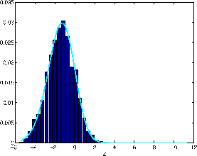Figure 6 shows the null distribution of pseudo-z-statistics resulting from the constrained HRF analysis on the artificial null data in section 4. This distribution is not Normal, in particular it is asymmetric. We therefore model the non-activation distribution in the mixture modelling as a flipped and shifted Gamma distribution. Figure 6 shows the fit of a flipped and shifted Gamma distribution to the null distribution histogram. Recall that with an f contrast we only look at the positive tail of the distribution to find both activations and deactivations. Therefore, we model the activations and deactivations as a single class in the spatial mixture modelling using a straightforward Gamma distribution.

Figure 6: Null distribution of pseudo-z-statistics resulting from the constrained HRF analysis on the artificial null data in section 4. This is the same histogram as that shown in red in figure 5(a). Also shown is the fit to this histogram of a flipped and shifted Gamma distribution.