Taking into account the autocorrelation

If we suppose $V \neq I\!d_T$ one will have to estimate it. If the estimate is ``good enough'', the estimates using GLS (sometimes called the EGLS for Estimated GLS or Empirical GLS, or plug-in estimated or two-stage least squares) will be good as well (nearly BLUE)¹⁹. It might be difficult to obtain a good estimate (estimating $V$ is estimating $T(T-1)/2$ parameters), so precluding the estimated-GLS²⁰ approach unless a model for the autocorrelation or $\sigma^2V$ in general can be made, reducing the number of parameters to estimate. The pre-whitening approach is in fact the EGLS approach; usually $V$ is modelled, for example, as an autoregressive process to have fewer parameters to estimate, as in Bullmore et al.(1996)[1]. 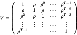For example let $\epsilon_t$ be an autoregressive process of order 1; $\epsilon_t=\rho\epsilon_{t-1}+e_t$ with $e_t$ as a white noise. Then the correlation matrix $V$ takes the form (exponential model):

$$V=\left ( \begin{array}{c c c c c} 1 &\rho & \rho^2 &\cdots... ...ots & \vdots\\ \rho^{T-1}& & & \cdots&1 \end{array} \right )$$ (23)

$$\mbox{ then } V^{-1}=1/(1-\rho^2)\left ( \begin{array}{c c ... ... 0& & & \cdots&1 \end{array} \right )=1/(1-\rho^2)^t\psi \psi$$

$$\mbox{ with }\sqrt{1/(1-\rho^2)} \psi=\left ( \begin{array}{... ...ots & \\ 0 & \cdots& & -\rho &1 \end{array} \right )=K^{-1}$$

where $\rho$ is going to be estimated, for example, on the residuals after a first stage least squares ( $\hat{\rho}=\sum_2\epsilon_i \epsilon_{i-1}/\sum_1 \epsilon_i^2$) or by fitting an exponential model onto the autocorrelogram. Classical time series analysis will allow estimations for autoregressive processes with higher order of dependence. GLS (or EGLS) uses $\hat{V}^{-1}$ and so can be very sensitive to a poor estimation of the correlation structure. Pointing out this problem, Worsley and Friston et.al(1995)[17] chose another way to take into account the autocorrelation. The GLM model can be written: $y=X\beta+K_Ie=X\beta +\epsilon$, with $e$'s uncorrelated, so that $var(\epsilon)=\sigma^2K_I{\;}^tK_I=\sigma^2V_I$. Their ``shaping approach'' uses the assumption that their chosen matrix filtering $K_{ij}=e^{[-(i-j)^2/2\tau^2]}$ (with a chosen $\tau$) will swamp the autocorrelation, $i.e.$ $KK_I \approx K$ where $K_I$ would give the true unknown one. Under this assumption the model is then written $y'=X'\beta +K \epsilon \approx X'\beta +Ke=X'\beta+\epsilon'$ with notations $y'=Ky$ and $X'=KX$. Deriving an OLS estimate gives an unbiased estimate but not BLUE anymore:²¹

$$\hat{\beta}=(^tX'X')^-{\;}^tX'y'$$

with variance

$$var(\hat{\beta})=\sigma^2(^tX'X')^-{\;}^tX'V X'(^tX'X')^-$$ (24)

given that now

$$var(\epsilon')=\sigma^2V= K var(\epsilon){\;}^tK=K V_I{\;}^tK=\sigma^2KK_I{\;}^tK_I {\;}^tK \approx \sigma^2K{\;}^tK$$ (25)

To estimate $\sigma$ they use the same formula as described in the previous section (equation (20) but with an OLS optimisation): $\hat{\sigma}^2=\frac{^t\epsilon'\epsilon'}{tr(P_{X'^\bot}V)}$ where $P_{X'^\bot}=I\!d_T -P_X'$ and $P_X'=X'(^tX'X')^-{\;}^tX'$. The $t_o$ map derived in the previous section is then used with the effective degrees of freedom²² calculated using classical results on quadratic form theorems [12]:

$$edf=\frac{2E(SS)^2}{var(SS)}= trace(P_{X'^\bot}V)^2/trace(P_{X'^\bot}VP_{X'^\bot}V)$$ (26)

The distribution of $\hat{\sigma}^2$ is approximatively ²³ distributed as $\chi^2_{edf}$ which then makes an approximate $t_{(edf)}$ distribution for $t_o$. Notice in this presentation, without ``swamping", setting $K=K_I^{-1}$ brings you back to GLS (see previous section). Within this debate of accounting for autocorrelation in fMRI, Woolrich et al. [16] propose a robust estimate $\widehat{V_I}$ of the autocorrelation of the time series. This robust estimate is then used either to pre-whiten the data (GLS) or to do an OLS estimation ($i.e.$ classical OLS under a non Gauss-Markov assumption²⁴) with filtering (as in Worsley and Friston's paper but without the swamping assumption) or without filtering (therein called variance correction) . The robustness is achieved in two ways, firstly by smoothing the non-parametric autocorrelation function for each voxel and secondly by smoothing the estimate spatially in a non-linear fashion to be able to preserve different patterns according to different matter types. Remark: Notice that a better estimate of $\sigma^2$ would have been using the form:

$$\frac{{}^t \epsilon' V^{-1}\epsilon'}{trace({}^t P_{X'^\bot}V^{-1}P_{X'^\bot}V)}$$ (27)

as given in equation (20) (here not with the BLUE), which uses the inverse of $V$ which Worsley and Friston wanted to avoid, but this time $V$ is given (Worsley and Friston) or is a robust estimate (Woolrich et al.) It seems that having a robust estimate of $V$ would incline one to use a GLS approach (pre-whitening). Note that in the last version of SPM'99 (Friston et al.) the ``swamping'' idea is dropped and an AR(1) model is used to estimate $V_I$. As this paper is written Friston[8] investigated the problem of estimating $V_I$ and choosing a filter in order to minimise the bias of (24). It is known that using an unbiased estimate $\widehat{V_I}$ for plug-in GLS estimation (EGLS) leads to good results for point estimation ( for $\beta$) but to underestimation for $var(\widehat{\beta} \setminus \widehat{V_I})$ (plug-in GLS variance), and more problematic underestimation of the true variance [2] of $\widehat{\beta}_{GLS}$, i.e. knowing $V_I$. So using OLS variances with a well chosen filter and a sensible estimate of $V_I$ would allow to obtain a more sensible estimate of the variance of $\widehat{\beta}$. If $V=I\!d_T$, i.e. no auto-correlation, or within the GLS framework, $edf$ is then equal to $T-rank(X)$, as seen before.